Reinforcement Learning Problems

Introduction to Reinforcement Learning

The objective in Reinforcement Learning is to find ways for an agent to learn to make good sequences of decisions. We indicate to the agent which action is good or bad with a reward function, and formulate the learning problem as an optimization problem that maximizes the total expected cumulative reward.

In order to maximize the total cumulative reward in a sequence of decisions, the agent may be required to balance immediate and long term rewards (and the future rewards’ uncertainty), which may require strategic behavior. This uncertainty can be rooted in the stochastic world or in the partial observed world.

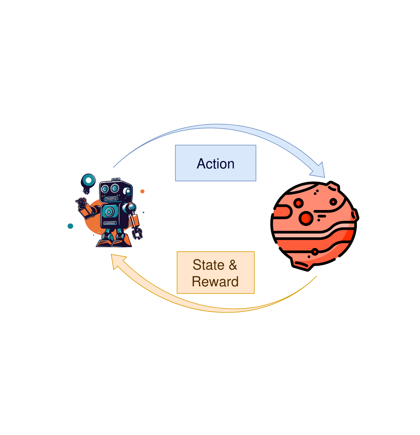
The agent behaves in an interactive closed-loop process, where it first performs an action given the current state, and then it receives the reward and the next state. This closed-loop behavior is possible under the Markov Assumption.

Markov Decision Process

The Markov Assumption is based in the concept of conditional probability, which is the chance of an event occurring given that a different event has already happened. In statistical terms, the Markov assumption tells us that the conditional probability of the future state, taking into account both the present and past states (or state-action tuples), is identical to the conditional probability of the future state given the present state (or present state-action tuple).

\[\begin{equation} P(s_{t+1}|s_t) = P(s_{t+1}|s_t,s_{t-1},s_{t-2},\dots, s_0) \label{eq:markov_chain} \end{equation}\]

This simplification is the basis for the Reinforcement Learning algorithms, because it removes the burden of keeping track of every state the agent has experienced up to the moment. In practice, we rarely think about the Markov Assumption, however, it’s influence in the RL algorithms turns it into a required topic to mention.

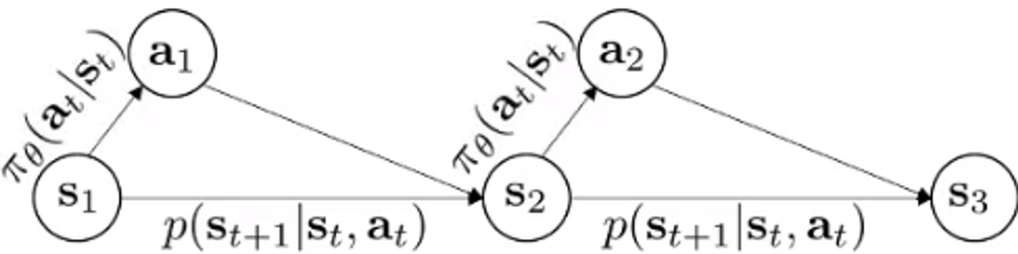
When we apply the Markov Assumption to a sequence of states, we get a Markov Chain. However, the chain only represent automatic transitions between states.

Instead, if we condition the next state with the current state and action, we create a Markov Decision Process. This formulation allows to introduce a mapping between the current state and the action, which is called the policy.

Some of the most important concepts of a Markov Decision Process are:

• S - state space → input for the agent
• A - action space → output for the agent
• T - transition/dynamics model → state transition probabilities conditioned on state-action pairs
• r - reward function → function that maps the current state and action into a reward value. It allows to define the objective

Introduction to Reinforcement Learning Algorithms

If we assume that our policy is a function approximator parameterized by a parameter vector $\theta$, we can formulate the RL objective as:

\[\begin{equation} \theta^* = \arg \max_\theta E_{\tau\sim p_\theta(\tau)}[\sum_t r(s_t,a_t)] \label{eq:rl_obj} \end{equation}\]

The above equation describes the RL problem as an optimization where we try to find the parameters θ that maximize the expected cumulative reward. To achieve this, the RL algorithms are normally composed of 3 components:

• Dynamics Model: Its the agent’s representation of how the world changes.
• Policy: Function mapping agent’s states to actions.
• Value Function: Function that outputs the cumulative reward by starting in a state (or state-action pair) and then following a particular policy. It is usually used to evaluate the value of a policy.

Usually, the difference between RL algorithms is defined by which of these components we try to learn and how we try to learn it. The 4 main types of RL algorithms are:

• Policy Gradients: Directly differentiate the objective above with respect to θ and then perform gradient descent.
• Value-based: Estimate a value function and use the estimated values to choose the best action (implicit policy).
• Actor-Critic: Estimate a value function and use it to evaluate and improve the policy (hybrid between policy gradients and value-based).
• Model-based RL: Estimate the transition/dynamics model, and then use it for optimal control or to improve the policy.

Value-based: Q-Learning

Q-learning is a value-based algorithm used to solve the RL problem. This method centers around the Q-function. This function returns the expected cumulative reward under a specific policy, conditioned on a state-action pair:

\[\begin{equation} Q^\pi(s_t,a_t) = \sum_{t=t'}^T E_{\pi_\theta}(r(s_{t'},a_{t'})|s_t,a_t) \label{eq:q_func} \end{equation}\]

Fundamentally, this means that the Q-function can be used to compare the goodness between two actions performed in the same state. If we can successfully represent the Q-function, then our agent can be an implicit greedy policy that chooses the action that maximized the Q-function in each state:

\[\begin{equation} \pi(s) = \arg\max_a Q^\pi(s,a) \label{eq:greedy_p} \end{equation}\]

However, how do we learn the Q-function?

Bootstrapping

Bootstrapping is a technique used in various fields, not just Reinforcement Learning. It essentially means using your current knowledge or estimates to improve and refine your future knowledge or estimates. In simple terms, it’s like pulling yourself up by your bootstraps, where your initial knowledge serves as a starting point to gain more accurate information or make better decisions.

In the case of Q-learning, we use the estimate of the Q-value of the next state to update the estimate of the Q-value of the current state, following the Bellman equation:

\[\begin{equation} Q^\pi(s_t,a_t) = r(s_t,a_t) + \gamma \max_a Q^\pi(s_{t+1}, a_{t+1}) \label{eq:bootstrap} \end{equation}\]

where $r$ is the reward function and $\gamma$ is temporal discount factor in order for the agent to prioritize rewards now more than later. This method is appealing because it is easy and fast to implement, however, because we are using wrong estimation to update our estimation, the Q-function usually accumulates some sort of bias. Even worst, this method only has convergence guarantees if our Q-function is of tabular form. For function approximators, such as neural networks, there are no theoretical guarantees. Despite that, algorithms using Q-learning tend to achieve good results in practice.

Deep Q-Learning Problems

Deep Q-Learning algorithms (using Deep Neural Networks) have some problems that can lead to poor results or train instability. However, some of these problems have some algorithmic design choices that helps to mitigate them. THe principal problems are:

• Maximization Bias: The maximization bias is induced by the maximization of the Q-function in the Bellman equation. Using a function approximator, the Q-function is approximated with an error that is evenly distributed to the positive and negative direction. When we choose the Q-value of the action that maximizes the Q-function, we are always choosing Q-values with a positive error (overestimating the Q-value). This produces a Q-function approximator that could greatly overestimate the value of some action, and, by the nature of bootstrapping, lead to instability in training. The solution to this problem is Double Q-Learning, where we learn 2 Q-function approximations and update one with the maximum of the other. Because of the random nature of the approximation errors, this de-correlation has good results

\[\begin{equation} \begin{aligned} Q_1^\pi(s_t,a_t) = r(s_t,a_t) + \gamma \max_a Q_2^\pi(s_{t+1}, a_{t+1}), \\ Q_2^\pi(s_t,a_t) = r(s_t,a_t) + \gamma \max_a Q_1^\pi(s_{t+1}, a_{t+1}) \end{aligned} \label{eq:dqn} \end{equation}\]

• Running Target: When training a function approximator to fit a Q-function, normally we define a target $y$ [eq. \eqref{eq:target}], and then perform supervised regression (usually with Mean Squared Error Loss) in order for the approximator to learn the right values. However, this procedure has a problem. Because the ground truth depends on the NN, after each update, the value of y for a given state-action sample can change drastically, creating a running target problem. The NN tries to catch up to the target, but target is always changing because the NN itself is always changing. This can lead to instabilities in training and poor convergence properties. The normal solution is the use of target networks. This target network is initialized with the same weights as the original. During training, only the original is updated with gradient descent, but the target y is calculated with the target network. The target network stays fixed, so the running target problem is mitigated. Lastly, for improvement’s sake, periodically, the weights of the original network are copied to the target network.

\[\begin{equation} y_i=r_j+\gamma\max_{a'_j}Q(s'_j,a'_j) \label{eq:target} \end{equation}\]

• Catastrophic Forgetting: Usually, in tabular formulation of Q-learning, the agent observes a state, takes an action, and then observes the reward and the next state $(s, a, r, s’)$. After observing this transition, the algorithm updates the values on the table using the Bellman equation. However, updating a NN using only one samples (batch size of 1) can lead to poor results. In Deep Learning, updating the NN using only one sample can lead to the forgetting of previously learned information. For these reason Deep Q-learning usually implements a replay buffer. This buffer stores a number of the last transitions experienced. At each network update, we sample uniformly a batch of transitions to perform gradient descent. This greatly reduces the effects of catastrophic and improves the stability and convergence capabilities of Deep Q-Learning.