Autoencoder: MNIST

Introduction

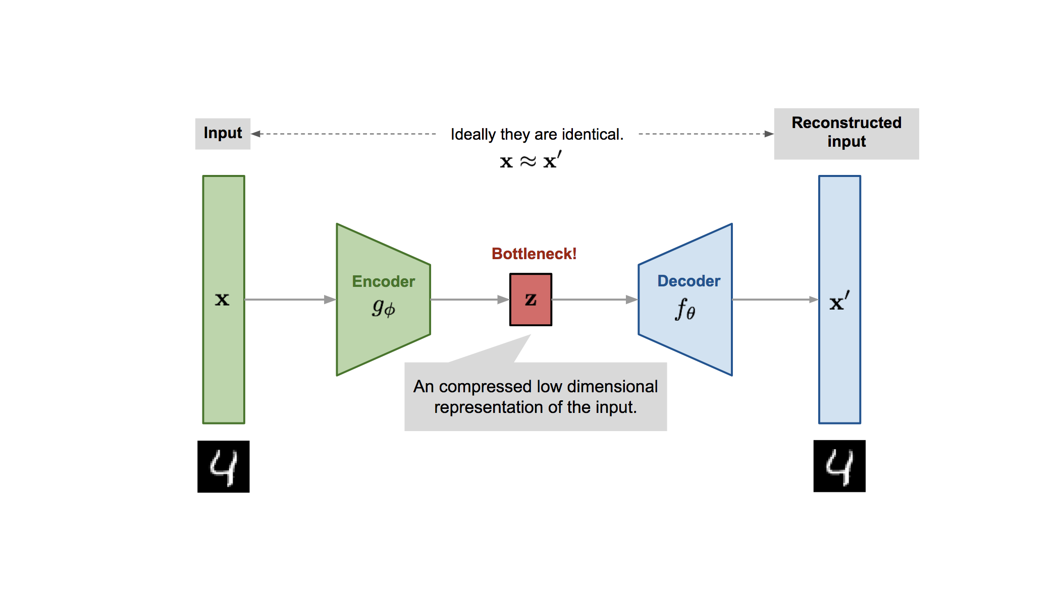
Typically, an autoencoder is a type of neural network used to reduce the dimensionality of data by projecting it onto a lower-dimensional manifold. This is achieved through a network architecture where the number of inputs matches the number of outputs, with a latent space (or bottleneck) that determines the extent of dimensionality reduction. Dimensionality reduction has a wide range of applications in machine learning. In control systems, for example, reducing the state space by eliminating redundant information can significantly enhance algorithms designed to explore that state space. A practical example is image compression, where an autoencoder can create a compact representation of an image that can be leveraged for downstream tasks such as classification, prediction, and control.

For these experiments, I will use the MNIST dataset, which is simple enough for rapid experimentation yet complex enough to test the effectiveness of compression algorithms.

Following the concepts from Bishop’s Deep Learning: Foundations and Concepts (link), we have chosen to test three types of deep autoencoders: a baseline autoencoder, sparse autoencoders, and denoising autoencoders. Both sparse and denoising autoencoders are relatively simple to implement and aim to learn more generalized representations of the data.

Autoencoders Overview

An autoencoder can be understood as two distinct mapping functions. The first function, $F_1$, is the encoder, which maps an input of size $D$ to a latent space of size $M$. The second function, $F_2$​, is the decoder, which performs the inverse mapping, reconstructing the original high-dimensional input from the latent space. In the case of neural networks, these encoder and decoder functions consist of layers of neurons interspersed with non-linear activation functions. Using neural networks allows us to capture non-linear structures in the data, something traditional methods like PCA (Principal Component Analysis) cannot do.

The way we train a Deep Autoencoder is by using backpropagation over the Mean Squared Loss

\[\begin{equation} E(w) = \frac{1}{2} \sum_{n=1}^N ||\Phi(x_n, w) - x_n||^2 \label{eq:msel} \end{equation}\]

where $\Phi$ is the autoencoder parameterized with weights $w$, and $x_n$. This loss is usually called Reconstruction Loss in image reconstruction.

In the case of images, autoencoders can often compress the data into a lower-dimensional representation because of the redundancy in pixel arrangements. For instance, when dealing with handwritten digits, there is a structured pattern to the way numbers are written. This means that less information needs to be stored since much of the pixel information is redundant.

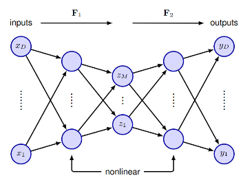Fig 1: Typical architecture for Deep Autoencoder (link)

Sparse Autoencoders

In the context of neural networks, a sparse representation means that only a small number of neurons in the latent space are “active” (i.e., have non-zero values) for a given input. In other words, for each input, most of the latent neurons remain “off” (outputting values close to zero), while only a few are “on.” There are several ways to enforce sparsity in the latent representation, but one of the simplest methods is to apply L1 regularization to the latent vector. This involves adding a component to the loss function that is proportional to the sum of the absolute values of the elements in the latent vector, as shown in equation \eqref{eq:sparse}.

\[\begin{equation} \tilde{E}(w) = E(w) + \lambda\sum_{k=1}^K|z_k| \label{eq:sparse} \end{equation}\]

Essentially, we are penalizing the model for having many active neurons in the latent space. The idea is that the model will attempt to minimize this penalty by encoding the same amount of information using fewer active neurons, thereby making the latent vector more sparse. This means that, although our autoencoder has a fixed latent space size of $K$, it will aim to represent the data using fewer neurons, effectively encoding the data in a space smaller than $K$. This adaptability allows for a more efficient representation of the data and addresses the limitation of neural networks with fixed layer sizes. Concept: Explain the difference between sparse autoencoders and traditional autoencoders, focusing on sparsity constraints and how they help in learning better feature representations. Mathematical Details: Include a brief explanation of how sparsity is enforced, such as L1 regularization or KL divergence.

Adding Noise (Denoising Autoencoders)

Denoising autoencoders are a type of autoencoder that learn to remove noise from input data. Typically, we add noise to the input (e.g., Gaussian noise) and then train the autoencoder to minimize the reconstruction loss by comparing the output to the original, noise-free input, as shown in equation \eqref{eq:noise}.

\[\begin{equation} E(w) = \frac{1}{2} \sum_{n=1}^N ||\Phi(\tilde{x}_n, w) - x_n||^2 \label{eq:noise} \end{equation}\]

Interestingly, this technique can have a similar effect to that of a sparse autoencoder, as it encourages the model to learn a richer, more descriptive representation of the data. By focusing on the denoising task, denoising autoencoders are forced to identify the most important features in the data in order to accurately reconstruct the original input. This results in a more invariant and generalizable representation. Moreover, this approach has the added benefit of simulating the types of noise often found in real-world data, making the neural network more robust and better suited for practical applications.

Experiments

In the following experiments, the autoencoders used are all instances of the class defined in the script below. The class is thoroughly commented for better understanding. This implementation allows us to test three methodologies by simply adjusting a few input parameters. For instance, to test a denoising autoencoder, we set randomize_input = True and specify the desired values for mean and std. To implement a sparse encoder, we can pass a sparse_lambda greater than zero.

As you may have noticed from the theoretical formulation of these encoders, as well as their instantiation, the parameters mentioned above do not affect the structure of the layers. Therefore, these methodologies do not alter the size or shape of the neural network. This consistency allows for a fair comparison between the methodologies while maintaining a fixed network architecture.

import torch 
from torch import nn

# Define a class for the Autoencoder Model using Multilayer Perceptron (MLP)
class MLP_AUTOENC(nn.Module):
    # The constructor (__init__) is used to initialize the model with various parameters
    def __init__(self, lr, input_dim, latent_dim, encoder_layers, decoder_layers, 
                 use_spectral_norm = False, use_bn = False, use_layer_norm = False, 
                 randomize_input = False, mean = 0.0, std = 0.1, sparse_lambda = 0.0
                 ) -> None:
        # Call the constructor of the parent class (nn.Module)
        super().__init__()

        # Set parameters for adding noise to the input
        self.mean = mean   # The mean of the Gaussian noise
        self.std = std     # The standard deviation of the Gaussian noise
        self.randomize_input = randomize_input  # Whether to add random noise to the input
        self.sparse_lambda = sparse_lambda  # Regularization parameter for enforcing sparsity
        
        # Define the encoder part of the autoencoder using a separate MLP class
        self.encoder = MPL(input_dim, latent_dim, encoder_layers, use_spectral_norm, use_bn, use_layer_norm)
        
        # Define the decoder part, which reconstructs the input from the compressed latent space
        self.decoder = MPL(latent_dim, input_dim, decoder_layers, use_spectral_norm, use_bn, use_layer_norm)

        # Define the optimizer (Adam) used for updating the model's parameters during training
        self.optim = torch.optim.Adam(self.parameters(), lr=lr)

    # Forward pass: defines how the data flows through the network
    def forward(self, x):
        # Optionally add random Gaussian noise to the input data if 'randomize_input' is True
        if self.randomize_input:
            x = self.addGaussianNoise(x)
        
        # Pass the input through the encoder to get the latent (compressed) representation
        red_vec = self.encoder(x)
        
        # Pass the latent representation through the decoder to reconstruct the input
        output = self.decoder(red_vec)

        # Return both the reconstructed output and the latent representation
        return output, red_vec
    
    # Loss function: calculates how far the reconstructed output is from the original input
    def loss(self, x, x_hat, red_vec = None):
        # Mean Squared Error (MSE) loss function measures the difference between x (input) and x_hat (output)
        loss_function = nn.MSELoss()

        # Calculate the MSE loss between the original input and the reconstructed output
        loss = loss_function(x, x_hat)

        # If sparsity is enforced (sparse_lambda > 0), add an extra term to the loss based on the absolute values of the latent representation
        if self.sparse_lambda > 0 and red_vec is not None:
            loss += self.sparse_lambda * torch.sum(torch.abs(red_vec))  # This promotes sparsity in the latent representation

        # Return the total loss value
        return loss
    
    # Function to add random Gaussian noise to the input
    def addGaussianNoise(self, tensor):
        # Create Gaussian noise with the specified mean and standard deviation
        noise = torch.randn(tensor.size()) * self.std + self.mean
        
        # Add the noise to the input tensor
        noisy_tensor = tensor + noise
        
        # Clamp (limit) the noisy tensor values to be between 0 and 1
        noisy_tensor = torch.clamp(noisy_tensor, 0., 1.)

        # Return the noisy tensor
        return noisy_tensor

# Define the class for the Multilayer Perceptron (MLP), used as both encoder and decoder
class MPL(nn.Module):
    # Constructor for the MLP class
    def __init__(self, input, output, hiddens, use_spectral_norm = False, use_bn = False, use_layer_norm = False) -> None:
        # Call the parent class constructor
        super().__init__()
        
        # List to store the layers of the MLP
        layers = []

        # Track the current input dimension for the layers
        current_dim = input

        # Loop through the hidden layer dimensions and add layers to the model
        for idx, hidden_dim in enumerate(hiddens):
            # Add a fully connected (linear) layer from current_dim to hidden_dim
            layers.append(nn.Linear(current_dim, hidden_dim))
            
            # Apply spectral normalization to the layer if specified
            if use_spectral_norm:
                layers[-1] = nn.utils.spectral_norm(layers[-1])
            
            # Apply batch normalization if specified
            if use_bn:
                layers.append(nn.BatchNorm1d(hidden_dim, affine=True))
            
            # Alternatively, apply layer normalization if specified
            elif use_layer_norm:
                layers.append(nn.LayerNorm(hidden_dim, elementwise_affine=True))
            
            # Add a ReLU activation function after the linear layer
            layers.append(nn.ReLU())

            # Update current_dim for the next layer
            current_dim = hidden_dim
        
        # After the hidden layers, add the final output layer
        layers.append(nn.Linear(current_dim, output))
        
        # Store the layers as a sequential model
        self.layers = nn.Sequential(*layers)

    # Forward pass for the MLP: pass the input through each layer
    def forward(self, x):
        # Loop through the layers and apply each one to the input x
        for idx, layer in enumerate(self.layers):
            x = layer(x)
        
        # Return the final output after all layers have been applied
        return x

The architecture used is shown in Fig. 2, which includes the number of hidden layers, hidden neurons, and the latent dimension. We opted for a small network to make the problem more challenging for the model to learn, allowing us to assess whether the denoising and sparse methodologies contribute to solving the problem.

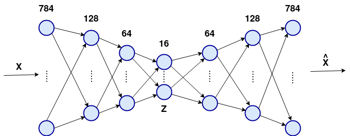Fig 2: Autoencoder architecture used in the experiments

The following table presents the remaining hyperparameters used, with some specific to certain methodologies.

Hyperparameter	Value
Learning Rate	0.0001
Batch Size	256
Epochs	100
Val Spit	30%
Batch Norm	True
Noise mean	0.0
Noise Std	0.2
Sparse Lambda	0.0001

Results

We now present the results of a training experiment for each methodology. While we are only showing one example, we performed many experiments to better understand the methodologies. Empirically, we found that the training instances do not vary significantly across experiments, so we can consider these selected experiments as representative.

Fig 3: Train and Validation loss of the baseline autoencoder 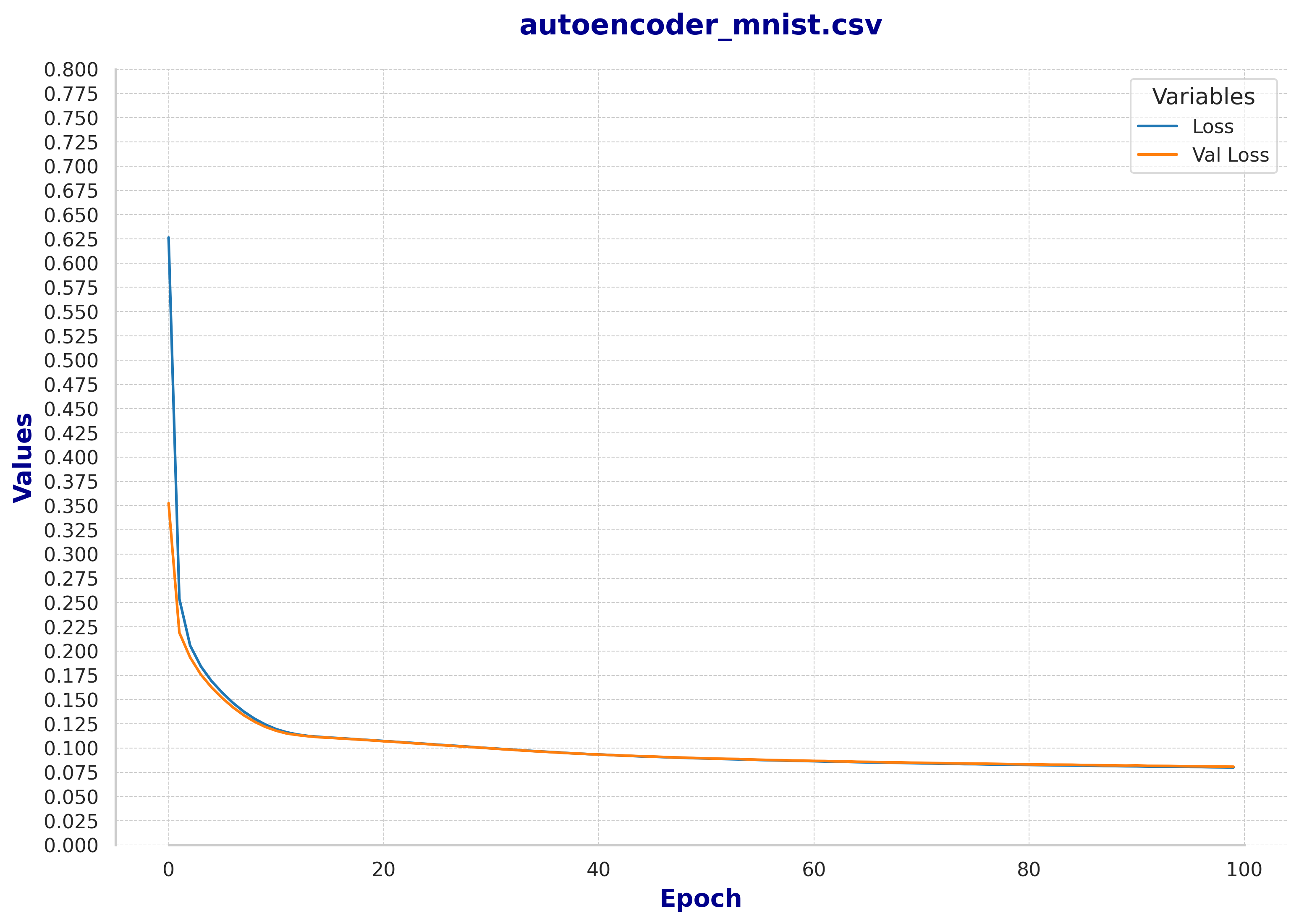Fig 4: Train and Validation loss of the denoising autoencoder 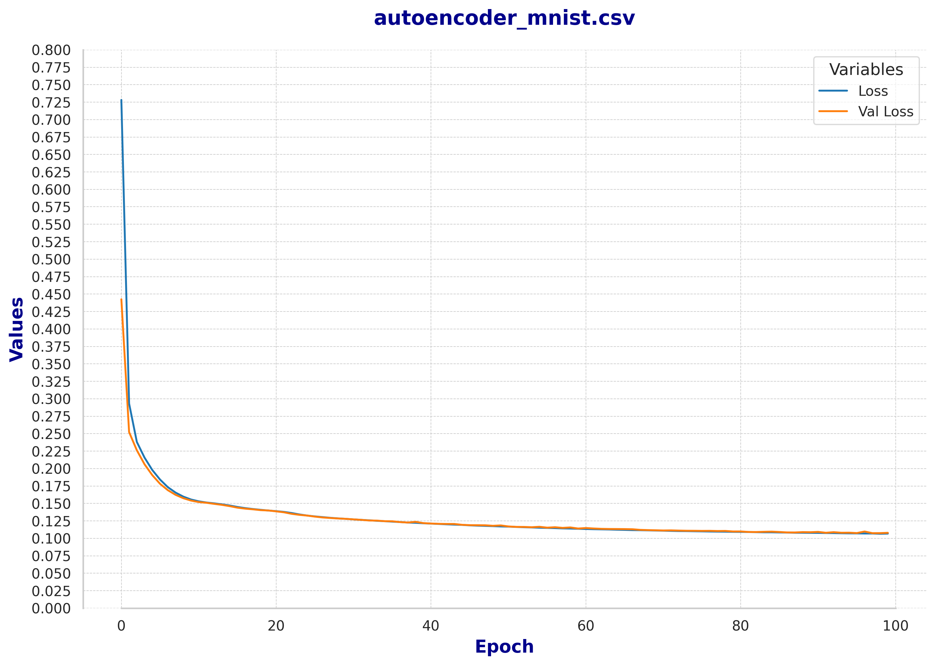Fig 5: Train and Validation loss of the sparse autoencoder

First, we can observe that after 100 epochs, the training process begins to stabilize. Although there are no signs of overfitting and, in theory, the loss would continue to decrease very slowly, we believe this is sufficient for a preliminary analysis.

An interesting qualitative analysis involves observing how some samples are reconstructed using the different methodologies.

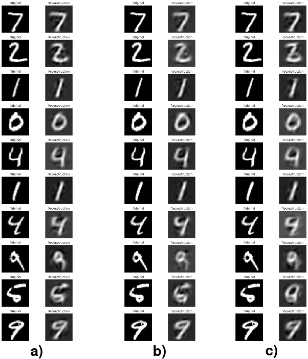Fig 6: Image reconstruction for: a) baseline, b) denoising autoencoder and c) sparse autoencoder

Discussion

First and foremost, we can conclude that the provided implementation is well-structured and can be confidently applied to more challenging scenarios. Additionally, the three methodologies employed yielded satisfactory results, especially considering that we were aiming for nearly 50-fold compression.

One interesting observation is that, based on the loss and reconstructed images, adding noise to the input did not seem to enhance the reconstruction task. Upon further investigation, we found that small networks may not benefit as much from the denoising technique. While denoising enables the network to capture more expressive structures in the data, the limited size of the network may prevent it from effectively learning those structures. There is also the possibility that the noise level was too weak, although we consider this less likely.

Another challenge was finding the appropriate value for lambda in the sparse implementation. A high lambda severely hindered the network’s ability to learn to reconstruct the images. This could also be due to the small network size. Since the sparse technique is intended to reduce the number of activations in the latent space, it might perform better with a larger latent space. The result was that, because the latent size was smaller than needed, applying the sparse regularizer only hindered the learning process. This is evident in the sampled reconstruction images, where we can observe that they are slightly worse.

Both of these techniques are typically regarded as training regularizers, which usually help prevent overfitting — an issue that arises when a network is larger than necessary. In hindsight, reducing the network size to its minimum may not have been the best approach for truly observing the effects of these methodologies.

Conclusion

In conclusion, Deep Autoencoders are a powerful tool, applicable to a wide range of machine learning tasks. Although our experimentation was limited, this implementation successfully solved the MNIST task. The primary goal of this implementation was to provide a sanity check for the code, ensuring it could be used in future projects, which it achieved.

However, we acknowledge that the comparisons between the baseline, sparse, and denoising autoencoders were not sufficiently conclusive. Therefore, we plan to continue experimenting with these techniques in the future.