Code Optimization: 8h to gain 26h
Introduction
This will be a short post that I was initially hesitant to write, but the insights and results from this experiment are valuable enough to document.
In essence, I spent about a day trying to figure out why my RL algorithm was running much slower compared to the baseline. Eventually, I managed to significantly reduce the computational time with relatively little effort.
Problem Identification
My algorithm is based on the Soft Actor-Critic (SAC) framework, with some additional features. Without delving too deeply into the specifics, my algorithm trains additional neural networks compared to standard SAC, which naturally increases computational requirements. However, in my specific use case and on my particular hardware, SAC completes training in 1 day and 5 hours (1d5h), whereas my algorithm takes 4 days and 5 hours (4d5h). This significant discrepancy cannot be explained solely by the addition of one extra neural network.
After profiling the execution times, I discovered that 65% of the runtime was consumed by the process of sampling transitions from the Replay Buffer. In my implementation, I use weighted sampling from the $(s,a,s′)$ transitions based on the cumulative reward, whereas standard SAC employs uniform sampling.
This process can be broken down into two key stages:
- Probability Calculation
- Sampling from the Buffer
The probability calculation operates as follows: given a buffer of returns $B_r$, my sampling process first determines the probabilities using the following equations:
\[\begin{equation} \begin{split} & m_r = \min(\min(B_r), 0) \\ & w_r = B_r + |m_r| \\ & probs = \frac{w_r}{\sum(w_r)} \end{split} \label{eq:probs} \end{equation}\]In essence, these equations ensure that if the minimum value in the buffer is negative, the values are shifted such that all become positive. Then, the adjusted values are normalized to sum to 1, resulting in a probability distribution for sampling.
Once the probabilities are calculated, transitions are sampled from the buffer without repetition, with the probability of selection directly proportional to the calculated probabilities. This approach is referred to as proportional sampling: samples with higher cumulative rewards are more likely to be selected, and this likelihood increases proportionally with their cumulative reward relative to the lower ones.
The issue with this formulation lies in its computational cost. Several operations in the process scale linearly with the size of the buffer. While linear time complexity is generally manageable, in this case, the buffer contains 1 million samples, and this code snippet is executed for each network update, amounting to 5 million iterations.
Clearly, we need a way to reduce the computational cost of these processes to improve efficiency.
Possible Solutions
In this section, I will discuss the solutions I tested during this experiment. While not all of these solutions were successful for my specific case, I believe it is still valuable to document them for future reference. My focus was on low-effort solutions that did not require extensive code refactoring. Additionally, some of the discarded solutions may indeed be effective, but I might not have fully understood how to implement them correctly.
Numba
Numba translates Python functions into optimized machine code at runtime. According to the examples provided, it can be as simple as decorating Python functions with a @jit() decorator, and it is compatible with many NumPy functions. However, in my case, the code became slightly slower than the original implementation, and some NumPy sampling functions were not compatible with Numba.
I also tried using the @njit(parallel=True) decorator, which is documented to enable parallelization. However, the code still utilized only a single CPU core, suggesting that parallelization might not have been applied successfully.
After spending about two hours reading the documentation and experimenting with various configurations, I concluded that the learning curve for effectively using Numba was somewhat steep. I decided to revisit it only if other options failed to yield better results.
C++ with PyBind11
Pybind11 is a header-only library that bridges C++ and Python, allowing C++ functions to be called directly within Python code, provided the C++ code is correctly written and compiled.
While this approach is fascinating and a valuable skill for running C++ code in Python, it did not yield benefits in this specific use case. Surprisingly, the C++ function called via Python was slower than the equivalent NumPy implementation. For context, NumPy itself is implemented in C++. However, since NumPy is a general-purpose library, one could argue that a specialized C++ function might outperform a general-purpose one in terms of speed.
This expectation was not met; the Python binding implementation ended up slower than NumPy. The reasons could include a lack of optimization in my C++ implementation or the overhead of the Pybind11 conversion process, which might have been significant enough to offset the performance gains of using C++.
After spending some time experimenting and given my limited knowledge of C++, I decided to revisit this option only if the other alternatives did not work.
PyTorch
Pytorch is an optimized tensor library designed for deep learning, supporting both GPU and CPU computation. Similar to NumPy, it is also implemented in C++. In my codebase, I was already using PyTorch to train the neural networks, while the rest of the RL management was handled with NumPy, inspired by the design of Gymnasium. This made the transition to PyTorch relatively straightforward and almost seamless.
As a library specifically built for tensor manipulation and machine learning, PyTorch includes the necessary statistical functions required for my implementation. This modification had the most significant impact on reducing computational time, as will be demonstrated in the following sections.
An interesting observation was that the code became slower when utilizing the GPU. My intuition is that the process is too simple for GPU acceleration to provide a benefit; the overhead of transferring data between the CPU and GPU likely outweighs any computational gains. Using the GPU is more justifiable for computationally intensive tasks, such as calculating gradients during neural network updates.
Don’t repeat yourself
During this analysis, I also discovered an inefficiency in my implementation. For each sampling operation, I was recalculating the minimum value of the buffer, even though the buffer only changes by one value per iteration (eq: $\ref{eq:probs}$).
To avoid this redundancy, I implemented a simple optimization: maintaining the minimum value in a separate variable and updating it whenever a new sample is added to the buffer. If the new value is lower than the current minimum, the variable is updated; otherwise, it remains unchanged.
This approach eliminates the need to search through the entire buffer to find the minimum value during every training iteration, significantly improving efficiency.
Results
I will now present three tables summarizing the execution times for the two main processes and the total time taken for the weighted sampling operation. These tables compare the performance of the NumPy-based implementation (old) and the PyTorch-based implementation (new). The times shown represent averages from 1,000 iterations for each data point.
Due to time constraints, this study was conducted quickly, as more pressing tasks required attention. Consequently, we do not have performance results for the Numba and C++ implementations. However, based on prior observations, you can trust that these implementations were either comparable to or slower than the NumPy implementation in our case.
| Devices | Old time (s) | New time (s) | Ration | Reduction(%) |
|---|---|---|---|---|
| Home | 0.0069 | 0.00114 | 6.05 | 83.5 |
| Deeplar | 0.0244 | 0.00648 | 8.3 | 73.4 |
| Larcc | 0.00647 | 0.000930 | 6.96 | 85.6 |
Tab 1: Times for probability calculation across three different machines
| Devices | Old time (s) | New time (s) | Ration | Reduction(%) |
|---|---|---|---|---|
| Home | 0.0174 | 0.0073 | 2,38 | 58.0 |
| Deeplar | 0.0168 | 0.00905 | 1.85 | 46.1 |
| Larcc | 0.0135 | 0.00675 | 2.00 | 50.0 |
Tab 2: Times for sampling from buffer across three different machines
| Devices | Old time (s) | New time (s) | Gained Time/Iter | Gained Time (h) | Ration | Reduction(%) |
|---|---|---|---|---|---|---|
| Home | 0.0243 | 0.00844 | 0.01586 | 22.02 | 2,88 | 65.3 |
| Deeplar | 0.0412 | 0.01553 | 0.02567 | 35.65 | 2.65 | 62.3 |
| Larcc | 0.0200 | 0.00768 | 0.01232 | 17.11 | 2.60 | 61.6 |
| Mean | 0.0285 | 0.01055 | 0.01795 | 26.38 (24.93) | 2.70 | 63.0 |
Tab 3: Times for total sampling process across three different machines. To estimate the time saved, we assume a total of 5 million iterations. We also highlight the mean time saved specifically for the two laboratory machines, as they will be used for training (the overall average, including all three machines, is provided in parentheses).
As we can see, the gains in computational time were remarkable, with the most significant impact observed on Deeplar, though substantial improvements were seen across all machines. In fact, we estimate a reduction of slightly more than a day in training time, bringing the total training duration down to 3 days.
While the original SAC still completes training in just 1.5 days, the additional delays are expected due to the new techniques and neural networks introduced in our implementation. It is also worth noting that weighted sampling will inherently take longer than uniform sampling, as it involves additional computational steps.
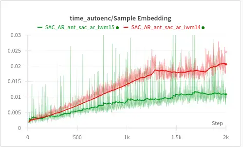
 Fig 1: A plot showing the time taken to sample transitions during training for the old implementation (red) and the new implementation (green).
In the previous plot, we validated the approach by running two identical training sessions, differing only in the weighted sampling implementation, on a generic test case. As training progresses, the time taken to sample transitions grows linearly, corresponding to the increasing buffer size.
Notably, the slope of the old implementation is steeper than that of the new implementation. Both approaches stabilize around the same time when the buffer reaches its maximum size of 1 million samples. However, the new implementation stabilizes at a much lower time compared to the old one, aligning closely with the values predicted by the isolated testing.
Conclusion
In this post, we discussed the time constraints imposed by weighted sampling in reinforcement learning. Our analysis showed that weighted sampling on a buffer containing 1 million entries consumed 65% of the total training time, compared to only 16% for uniform sampling.
After identifying this bottleneck, we implemented several changes to the codebase, with the most impactful being the transition to PyTorch. PyTorch demonstrated superior performance in matrix operations and probabilistic sampling, leading to significant efficiency gains.
As a result, we successfully reduced the total training time by approximately one day. This improvement allows us to conduct more experiments and further validate our hypotheses, driving progress in our research.
