Fetch Robot

Robot Description

The Fetch Robot is a mobile manipulator designed for human working environments (indoor). It has 13 DoF in total, with a mobile base, torso lift, 7-DoF arm, gripper and head. Fetch was created to aid research of mobile manipulation, and has a scientific paper justifying its contributions to the field. In this link we can find a detailed description of this device.

For now, the relevant information about the robot is:

-Arm: 7 revolute joints disposed perpendicularly in sequence. It is capable of lifting 6 kg in full extension. -Gripper: 2 fingers with linear movement with maximum opening of 100 mm. -Torso: 1 prismatic joint perpendicular to the base. The limits of the prismatic joint are not specified.

This is all the information that influences the position of the end effector, because the base of the robot will be fixed on the following experiments.

Environment Description

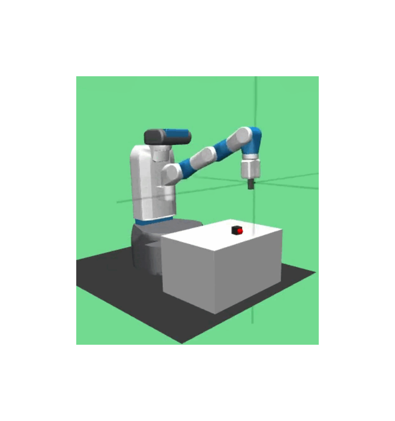
In these experiments we used the Gymnasium-Robotics library. This resource comes with built-in handful of environments (in MuJoCo) and tasks. In this post, we’ll focus on the Fetch Environment with the PickAndPlace task.

In this task, Fetch needs to learn how to pick a cube that rest on a random position on top of a table. After that, the robot needs to move the block to the goal represented as a red dot. The cover image of this post illustrates the task. We’ll describe the environment and task’s setup, however we also linked the official documentation before for a more detailed description.

Action Space

The action space corresponds to the outputs of the Reinforcement Learning agent. This space defines the way the agent interacts with the world, and can limit or bias its thinking. Therefore, the formulation of the action space can be deciding factor for the agent to accomplish or not a given task (especially in robotics).

In these experiments, the outputs of the RL agent are the small displacements of the end effector on the 3 Cartesian coordinates, and the absolute displacement of the gripper’s fingers. The gripper’s orientation is fixed in a perpendicular position relative to the table, always pointing down. Utilizing the fixed orientation and the small displacements $(dx, dy, dz)$, and the inverse kinematics computed internally by the MuJoCo Framework, the RL agent can control the robot.

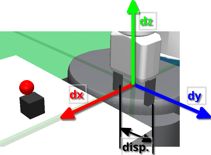Fig 1: Action Space representation

Observation Space

The observation (or state) space corresponds to the inputs of the Reinforcement Learning agent. This space defines the way the agent perceives the world. The formulation of a state space has two major requirements. Firstly, we need to always try to respect the Markov Assumption, because this is assumption is used in all the RL algorithms. Secondly, we need to guarantee that the agent is receiving all the information that is relevant to accomplish the task. We might also be aware that if the information is all relevant. Providing irrelevant information can complicate the learning process, however the agent could learn how to ignore it.

The observations space is a goal-oriented observation space. This means that the state vector has some entries that represent the state of the environment and other entries that represent the goal. In these experiments, the state vector has 31 dimensions (25 environmental + 6 goal). Environmental:

Environmental:

• End effector’s global position: 3 Cartesian coordinates of the end effector in the global frame.
• Block’s global position: 3 Cartesian coordinates of the block in the global frame.
• Block’s relative position: 3 Cartesian coordinates representing the difference between the gripper position and the block position (still in the global frame).
• Joint displacement of the gripper’s fingers: 2 values indicating the displacement of the fingers
• Block’ rotation: 3 XYZ Euler angles of the block’s rotation in the global frame
• Block’s relative linear velocity: 3 linear velocity components of the block in the gripper’s local frame
• Block’s angular velocity: 3 angular velocity components of the block in the global frame
• End Effector’s linear velocity: 3 linear velocity components of the end effector in the global frame
• End Finger’s linear velocity: 2 linear velocity components of the gripper’s fingers in the global frame

Goal:

• Block’s global position: 3 Cartesian coordinates of the block in the global frame. (repeated by mistake)
• Block’s global desired position: 3 Cartesian coordinates of the block in the global frame representing the goal.

In this environment we see a normal approach in robotics, to provide the agent with the positions and velocities of the robot, and some additional information regarding the objects of interest. We also choose data that it’s the direct computation of other values (eg. Blocks relative position). Although the agent could figure out these correlations by itself, sometimes it helps to give some additional (even redundant) information.

How to Complete the Task

The task is never complete, because we are training the agent in an infinite horizon setting. The reason is that we would like for the robot hold the object in position for an indefinite amount of time, which could be useful for a handful of task (eg. handover). However, although the task never stops, we can define a success condition. In this case, the success condition is achieved when the distance between the block and the goal position is less than 0.05 m.

Reward Description

The reward function is a crucial decision in RL problems. A well-defined reward function can do almost all the heavy lifting of the learning process, almost to the point where the choice of the RL algorithm becomes less important. However, highly specialized and complex reward functions can backfire, and the agent might learn to optimize the function in ways that don’t solve the task! Therefore, the tendency in the research community is to use more simplistic and general reward function (almost at the binary extreme of success/non-success). For this reason, we experimented with 3 different rewards:

• Sparse: At each time step, the agent receives a reward of -1 if the task is not successful, and 0 otherwise. This has the effect of motivating the agent to perform the task as quickly as possible. However, the sparse reward only gives meaningful feedback once the agent achieves the goal.
• Dense: At each time step, the agent receives a reward proportional to the negative distance between the blocks current position and desired position. This reward also has the effect to motivate the agent to perform the task as quickly as possible. However, the function also gives feedback every time the agent moves the block.
• Dense + Tool Distance: This reward function adds on the Dense function. In addition to have the negative of distance between the block’s current and desired position, we also add the negative of distance between the gripper and the block. The idea is to aid the agent in early stages of training to find the object faster and more consistently.

Algorithms

In these experiments, there were used two popular RL algorithms: Soft Actor-Critic (SAC) and Proximal Policy Optimization (PPO). These two algorithms are Actor-Critic, and are normally used for continuous settings (like robotics). We’ll not get into much detail on these algorithms (maybe in a different blog post), however we’ll discuss some important facts.

Firstly, these algorithms are very different from each other in design choices, and they both excel in different areas. SAC is an algorithm which focuses on exploration. Basically, when training the actor and the critic networks, SAC adds additional losses based on entropy to incentive the agent to choose less tested actions. This intuition behind this is Optimistic Exploration: unknown actions are good actions, in worst-case scenario we discover they are bad. This means that SAC is better at exploring, however it becomes more unstable because sometimes in can choose to explore the wrong path instead of following the wright one. This algorithm is an off-policy algorithm, which means that uses data points not collected by the current policy. For this reason, the SAC is more data efficient, but off-policy algorithms tend to be more unstable.

PPO is the complete opposite of SAC. This algorithm was created to be the most stable possible. PPO achieves this by being on-policy, which means that learning is performed with data points collected by the current policy. However, PPO loses data efficiency by being on-policy. Another property of PPO is that in each training step, it tries to stay close the current policy, only changing a bit. This means that, although PPO is more stable and monotonically improving, it can more easily settle for a local minimum that does not solve the task.

In conclusion, both PPO and SAC are actor-critic, which means that the neural networks architectures are practically the same. The difference between them is in the data used to train and how they calculate the losses to update the neural networks. For this reason, we proceeded to test both of them with the different reward formulations.

Results

In this section, we’ll discuss the results obtained training the agent with the algorithms and the reward functions discussed before. For each of the 6 combinations, we ran 3 different trains throughout 100 000 episodes. Each episode has 100 steps, which means that each algorithm has 10 000 000 data points of train. Additionally, there was no optimization of the algorithms and its hyperparameters. The lack of optimizations and the low number of runs makes it difficult to draw meaningful conclusions about the algorithms. However, the results may provide an interesting foundation to continue exploration in this topic.

In these experiments, we tried to maintain the train conditions between the two algorithms, with special attention to the number of data points collected (10 000 000). However, this approach may not be fair, because it puts PPO (which is more data inefficient) in a clear disadvantage. For comparison, PPO acquires 2 048 data points and then performs 10 gradient steps (learning steps) in that data. This means that, with 10 000 000 data points, PPO performs a total of around 48 900 learning steps. However, SAC performs a gradient step at each data point collected (by leveraging its buffer), which means it performs 10 000 000 learning steps. In conclusion, in our experiments SAC is 200x more efficient with the data. However, each SAC run took 2 days while each PPO run took 14h. This may indicate that in future experiments we give more data points to PPO than to SAC to compare them properly.

Accompanying each graph, there will be a video testing the best model achieved with the combination of algorithm and reward function. We’ll also present a small discussion justifying the results.

PPO - Sparse Reward

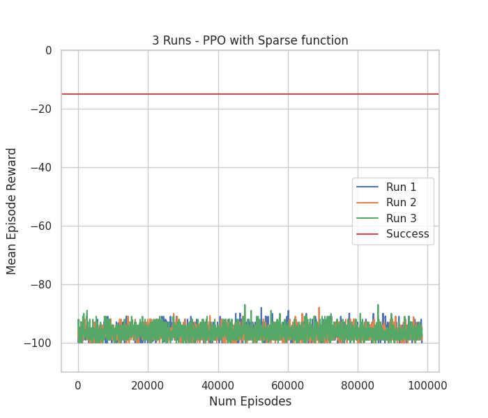Video testing 10 episodes with run number 1 & Figure with Mean Episode Reward
of 3 runs throughout 100 000 episodes of train

As expected, PPO with Sparse reward could not solve the task. The lack of meaningful feedback throughout each episode completely undermines the learning process, and PPO seems to not be able to deal with it. Moreover, we can clearly see in the video that the agent performs the same actions regardless of the observation. This implies that probably the agent would never learn to solve the task even if we let it run more time.

PPO - Dense Reward

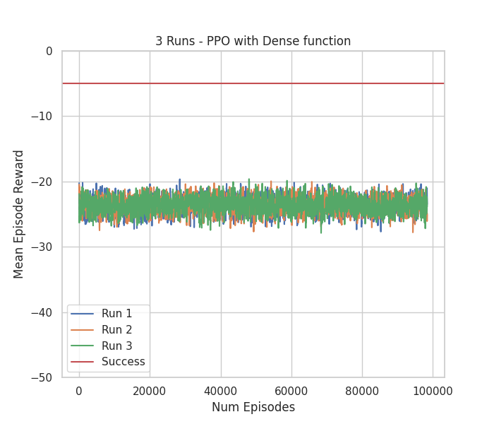Video testing 10 episodes with run number 2 & Figure with Mean Episode Reward
of 3 runs throughout 100 000 episodes of train

In this experiment, the Dense reward function seemed to not help PPO. As previously discussed, the Dense reward only provides meaningful feedback once the object is moved. This implies that PPO did not explore enough to reach that stage. Additionally, by the mean reward graph, we can conclude that the train would probably never converge if given more time.

PPO - Dense + Tool Dist Reward

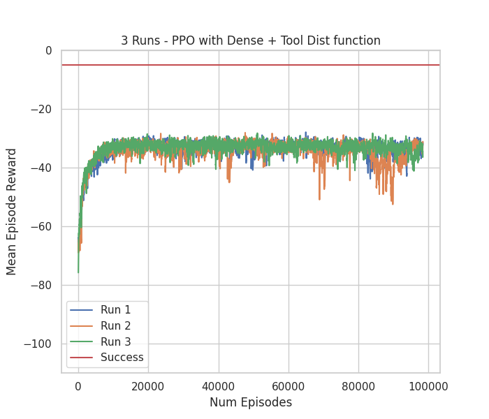Video testing 10 episodes with run number 1 & Figure with Mean Episode Reward
of 3 runs throughout 100 000 episodes of train

The additional reward component with the distance between the end effector and the block was proposed specifically to aid PPO in the first exploration stage. However, we did not achieve great results. In the video and graphs, we can see that PPO learned to optimize the Tool Dist component in way that became difficult optimizing the second component (the main task objective). This implies that we could do some fine-tuning to the reward components, by scaling them relative to each other. However, this technique adds more hyperparameters to an algorithm that is already hyperparameter heavy.

SAC - Sparse Reward

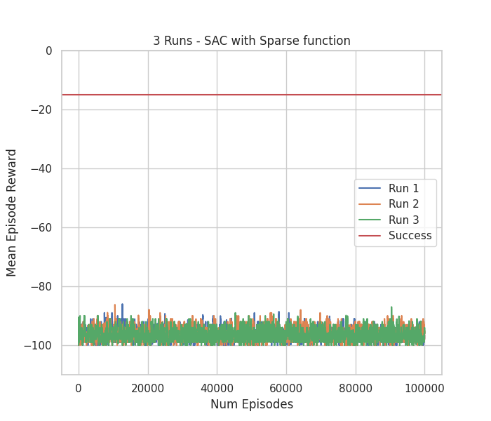Video testing 10 episodes with run number 1 & Figure with Mean Episode Reward
of 3 runs throughout 100 000 episodes of train

As expected, the SAC and Sparse reward combination could not solve the task. The problem of lack of meaningful feedback until the task is complete could not be overcome. However, we can see the exploratory nature of SAC in the video. We can see that the algorithm tries different actions for different states. Even without any reward signal, it tried to explore its environment. Lastly, we can also conclude that the algorithm would never converge with this experiment setup.

SAC - Dense Reward

Video testing 10 episodes with run number 1 & Figure with Mean Episode Reward
of 3 runs throughout 100 000 episodes of train

The combination of SAC and Dense reward was the only one that could solve the pick and place task. We can conclude that SAC leverage its exploration to find the block without any explicit motivation. After that, it could optimize the Dense reward by learning how to properly manipulate the block. There is some variation in the different runs (run number 1 converged faster), however we can conclude that this setup would almost always converge given enough time.

SAC - Dense + Tool Dist Reward

Video testing 10 episodes with run number 1 & Figure with Mean Episode Reward
of 3 runs throughout 90 000 episodes of train

Although the Tool Dist + Dense reward was proposed to help PPO, we also test it in SAC. Before testing, we would assume that this setup would be even better compared to using the Dense reward. However, the results show different conclusions. Firstly, none of the runs converged, and the graph progression suggests they would never converge. In the video, we can intuitively see that the agent got stuck in a local minimum that only optimized the first reward component (similar to PPO). These results reinforce the belief that creating more complex rewards could backfire, because we cannot foresee what effects it will have in the learning process.

Conclusions

In this blog post, we could not draw meaningful conclusions about the algorithms or the training setups. However, we learned a lot about Environment and Task definition, PPO’s and SAC’s behaviors and RL’s results analysis. This exercise also allowed us to develop a lot of tools to train, test and inspect the future RL problems. Therefore, in the conclusions of this post we suggest future work rather than discuss conclusions.

• PPO’s hyperparameter optimization: We believe that PPO should also be able to solve this task with the Dense reward, if we optimize its hyperparameters accordingly.
• Improve complex reward: We believe that SAC/PPO with Tool Dist + Dense reward should be able to solve the task. For this, we might need to scale the Tool Dist down to give it less importance.
• Causal Action Influence: We believe that strategies that improve exploration should help in this type of tasks, Therefore, we could follow a paper (already being implemented) where the authors used a measure of causal influence to motivate meaningful environment exploration.

If we can achieve these 3 bullets points, maybe we can close this chapter a move on to more realistic Environments and Tasks.