PPO Hyperparameter Optimization
Introduction
Expanding on our previous discussions about Proximal Policy Optimization (PPO) in reinforcement learning, let’s now focus on a crucial aspect: hyperparameter optimization. In reinforcement learning research, hyperparameters play a critical role in determining the effectiveness and stability of algorithms like PPO. Whether it’s adjusting learning rates, fine-tuning clipping parameters, or optimizing entropy coefficients, finding the right settings is essential for successful training. In this blog post, we’ll delve into the process of hyperparameter optimization specifically for PPO, providing insights to help you maximize its performance in various decision-making scenarios.
In a previous blog post, we explored the PickAndPlace task proposed by Gymnasium-Robotics. In that experiment, we found out that the PPO algorithm could not solve the task with any of the three reward functions. This seemed odd because PPO is a very powerful algorithm, and the complete guidance of the Tool Dist + Dense reward function should be enough to solve that task. This could mean that the chosen hyperparameters were not fit for the task, and we should conduct hyperparameter optimization.
In this section, we will describe the choices and considerations taken in this optimization process. Firstly, will lightly review the environment and reward setup used. After that, we will talk a bit about the optimization tool utilized, which is integrated in Weights and Biases. Following that, we’ll present the hyperparameters being optimized, the optimization ranges and the usual effect they have in PPO. Lastly, we’ll describe the evaluation metric used in the optimization.
First and foremost, we recommend reviewing the Fetch Robot post as the experiments discussed here will build upon the descriptions provided there. We will now briefly overview some of the more critical aspects; however, please note that this description will not be as extensive as the previous one.
The PickAndPlace task is a goal-oriented objective where the Fetch robot must pick up a cube from a table and relocate it to a random position either on the table or suspended in the air. Below, we present a video example of the task being completed. Despite the Fetch robot’s high level of redundancy, this environment restricts control to only four variables: the end-effector position (3) and the gripper displacement (1). Furthermore, the end-effector is constrained to maintain a perpendicular orientation to the floor, facing downward.
The utilized reward function is the Tool Dist + Dense. This reward comprises two components. The first component calculates the distance between the block’s position $B$ and the goal $G$. This component directly influences task performance and is thus considered the primary component. The second component measures the distance between the block’s position $B$ and the end-effector $E$. This aspect can be viewed as optimizing a sub-task aimed at locating the block, which is crucial for completing the main task. Consequently, we introduced a coefficient $\beta$ to scale down this component, reducing its significance relative to the primary task reward component. Throughout all our experiments, $\beta$ was consistently set to 0.5. Equation 1 formalizes the Tool Dist + Dense reward.
Weights and Biases: Sweep
Weights & Biases is a versatile machine learning platform designed to streamline model development for developers. With W&B’s lightweight and interoperable tools, users can effortlessly track experiments, manage dataset versions, evaluate model performance, replicate models, visualize results, detect regressions, and collaborate by sharing insights with colleagues.
W&B has a powerful tool named Sweep, that automates hyperparameter search and facilitates comprehensive experiment tracking. It offers various search methods, such as Bayesian, grid search, and random search, enabling systematic exploration of the hyperparameter space. Additionally, W&B provides visualization capabilities for experiment tracking, allowing users to monitor and analyze results effectively. Moreover, the platform supports scalability and parallelization across multiple machines, enhancing efficiency in parameter configuration exploration and optimization. Also, the implementation of the W&B functionalities is easily compatible with Python and the Reinforcement Learning libraries already used (Gymnasium-Robotics and Stable-baselines3).
In our experiments, we employed the Bayesian Hyperparameter Optimization method provided by the Sweep tool. This approach is known for its efficiency in discovering optimal solutions as it utilizes past information from the optimization process to make informed guesses about the location of optimal hyperparameters. For further insights into Bayesian Hyperparameter Optimization, you can explore this web article. Additionally, we frequently chose to discretize the values that the Optimizer could select. This strategy aimed to reduce the number of potential combinations and expedite the optimization process, particularly considering the substantial number of hyperparameters being optimized.
Hyperparameters
PPO is known to be a hyperparameter heavy algorithm. We decided to focus on optimizing 12 of these key hyperparameters. To make things easier, we narrowed down the possible values for each parameter based on insights from a relevant web article and the original PPO paper.
- Batch Size: $[32, 64, 128, 256, 512]$
- $\epsilon$ (clip range): $[0.1, 0.2, 0.3]$
- $c_2$ (entropy coefficient): $[0, 0.0001, 0.001, 0.01]$
- $\lambda_{GAE}$: $\mathcal{U}(0.9, 1)$
- $\gamma$: $\mathcal{U}(0.8, 0.9997)$
- $lr$ (learning rate): $[0.000003, 0.00003, 0.0003, 0.003]$
- log_std_init: $[-1, 0, 1, 2, 3]$
- epochs number: $[3, 6, 9, 12, 15, 18, 21, 24, 27, 30]$
- steps number: $[512, 1024, 2048, 4096]$
- normalize advantages: $[True, False]$
- target_kl: $\mathcal{U}(0.03, 0.003)$
- $c_1$ (value coefficient): $[0.5, 1]$
We also provide a table detailing a succinct description of each hyperparameter along with its anticipated impact on the PPO algorithm. This resource will be important in interpreting the outcomes of the optimization process.
| Hyperparameter | Description | Influence in PPO |
|---|---|---|
| Batch Size | The number of samples used in each training batch. | Larger batch sizes typically lead to more stable training but may require more memory and computational resources. |
| Clip Range | The threshold for clipping the ratio of policy probabilities. | Clipping the ratio helps to prevent overly large policy updates, ensuring stability during training. |
| Entropy Coefficient | A coefficient balancing between exploration and exploitation. | Higher values encourage more exploration, while lower values prioritize exploitation. |
| $\lambda_{GAE}$ | The parameter controlling the balance between bias and variance in estimating advantages. | Lower values increase bias but reduce variance, leading to more stable training but potentially less accurate value estimates. |
| Learning Rate | The rate at which the model’s parameters are updated during training. | A higher learning rate can accelerate learning but may lead to instability or divergence if too large. |
| Log Std Init | The initial value for the logarithm of the standard deviation of the policy. | A higher initial value can encourage more exploration in the early stages of training. |
| Epochs Number | The number of times the entire dataset is used during training. | Increasing the number of epochs allows for more passes through the data, utilizing data more efficiently. |
| Steps Number | The number of steps taken when accumulating the dataset. | More step numbers allow for more information to be gathered per iteration, potentially leading to more efficient and stable learning. |
| Normalize Advantages | Whether to normalize advantages before using them in training. | Normalization can help to stabilize training by scaling advantages to have a consistent impact on policy updates. |
| Target KL | The target value for the Kullback-Leibler (KL) divergence between old and new policies. | Adjusting the target KL helps to regulate the magnitude of policy updates, promoting smoother learning. |
| Value Coefficient | The coefficient balancing between the value loss and policy loss in the total loss function. | A higher value coefficient places more emphasis on the value function, potentially leading to more stable training. |
Evaluation Metric
The W&B Sweep associates a predetermined set of values for hyperparameters with a continuous output of our choosing. We have the option to either maximize or minimize this output according to our objectives. In our case, following each training iteration, we assessed the resulting policy across 100 episodes and computed the Mean Episode Reward. We determined that 100 episodes provided sufficient stability in the testing procedure. Subsequently, we configured the Sweep to maximize this value. Given the nature of the reward function as a cost of living, our objective is not only to identify a policy capable of solving the task but also to achieve the fastest solution in expectation.
Experiments
In this section, we will outline pertinent details regarding the optimization process, discuss the obtained results, and share valuable insights gathered throughout the experimentation.
Sweep Information
The optimization process ran continuously with 8 parallel training agents, completing a total of 209 runs over the course of 93 days of compute time. In real-time terms, the optimization process spanned 11 days, with the optimal hyperparameter values identified on day 7. It’s essential to emphasize that this was a significant computational cost, made feasible only with moderately good computing resources (LAR’s servers).
Each run performed 5,000,000 steps in the environment, equivalent to approximately 100,000 episodes. This number of episodes is notably smaller compared to experiments conducted in previous blog posts. The rationale behind this decision was that, even if a run did not complete consistently the task during the optimization process, the best run would likely accomplish the task given additional training time. Thus, we aimed to identify the best run while reducing computation costs by approximately 2-fold. Moreover, providing fewer steps for convergence (within reasonable values) favors runs that converge more quickly, which is a notable advantage.
Results
W&B Sweep creates a visualization that is shown in Figure 1. On the left side, you’ll find a plot depicting the Mean Episode Rewards achieved by the 209 runs. On the right side, the Sweep displays the correlations between the evaluation metric and hyperparameters, along with their respective importance.
 Fig 1: Optimization results. On the left side, you’ll find a plot depicting the Mean Episode Rewards achieved by the 209 runs. On the right side, the Sweep displays the correlations between the evaluation metric and hyperparameters, along with their respective importance.
As observed in left side of Figure 1, the initial runs yield episode reward values ranging between $[-30,-15]$, indicating that the task is not being effectively solved. However, the optimizer quickly suggests hyperparameters that lead to runs achieving episode reward values between $[-15,-10]$. Such values are attained only if the agent sporadically completes the task. Subsequently, we observe a run with an episode reward value of $-5$, suggesting consistent task completion across the 100 test episodes. This run was identified as the best run and its hyperparameters will be disclosed shortly. Additionally, it’s noteworthy that the evaluation points exhibit a linear trendline with a slightly positive inclination, signifying that the optimization process progressively improves over time. Perhaps, given more time, the Sweep would propose hyperparameters exclusively capable of solving the task.
On the right side of Figure 1, the importance and correlations of each hyperparameter to the evaluation metric are displayed. It’s evident that, overall, the learning rate emerges as the most influential hyperparameter across all runs, exhibiting a highly negative correlation. This indicates that to maximize the evaluation metric, decreasing the learning rate is necessary. Such a finding shouldn’t be unexpected, as smaller learning rates promote more stable learning, aligning with the primary objective of PPO.
However, we can delve deeper into our analysis by excluding the poor-performing outliers and concentrating solely on the good runs. This approach allows us to discern which hyperparameters differentiate the medium runs from the good ones. In Figure 2, we present the same analysis but exclusively with runs that attained an evaluation metric exceeding $-15$, totaling 165 runs.
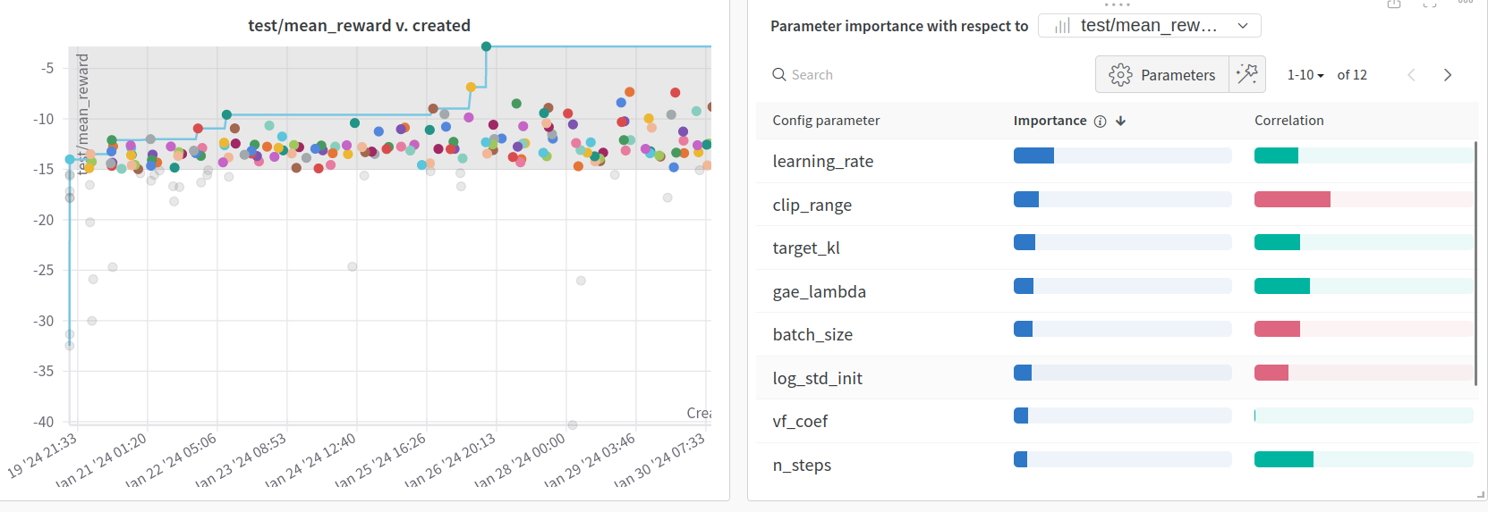 Fig 2: Optimization results of the 165 runs that obtain more that $-15$ Mean Episode Reward.
In this instance, we observe a significant decrease in the importance of the learning rate, although it remains the most crucial hyperparameter. Moreover, the learning rate now exhibits a positive correlation. This shift may be attributed to the fact that all runs reaching this stage possess the smallest available learning rates. Consequently, among the smaller learning rates, selecting the highest one may be advantageous. This concept aligns with the understanding of the learning rate in Deep Learning, where there exists an optimal value beyond which increasing or decreasing the learning rate deteriorates learning performance.
Furthermore, this analysis highlights two hyperparameters unique to PPO: clip range and target_kl. These hyperparameters play a crucial role in constraining the magnitude of policy updates during learning. Despite their contrasting correlations, their significance, along with that of the learning rate, underscores the importance of regulating policy updates for achieving consistent and stable learning performance.
Finally, we will examine the runs that achieved an evaluation metric greater than $-10$ to identify the hyperparameters distinguishing the good runs from the best ones. It’s important to note that we now have only 18 runs, which may not constitute a sufficiently large sample size to draw definitive conclusions, but we will still give it a shot.
 Fig 3: Optimization results of the 18 runs that obtain more that $-10$ Mean Episode Reward.
In this scenario, we can see in Figure 3 that the target_kl hyperparameter takes center stage with a positive correlation. A higher target_kl permits larger policy updates, facilitating faster learning. Considering that we capped the amount of data seen per run, it’s possible that the best runs exhibited larger target_kl values because they learned and converged more quickly, demonstrating greater data efficiency. Additionally, we notice the normalized advantage property, suggesting that normalizing the advantage could be beneficial as it promotes training stability.
After the hyperparameter optimization, we selected the best hyperparameter configuration and conducted four separate experiments using these parameters for 10,000,000 steps each. We then averaged the success rate curves of the four runs and plotted them in Figure 4, with the shaded area representing the variance across all the runs. This visualization provides an understanding of both the average performance and its variability.
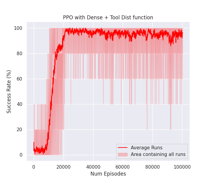 Fig 4: Average success rate curve throughout training of the 4 runs.
As evident from the graph, the selected hyperparameters not only yield a consistent success rate nearing 100%, effectively completing the task, but they also achieve this milestone in approximately 20,000 episodes, indicating rapid learning. Additionally, we observe minimal variance between runs, highlighting the stability characteristic of PPO.
- Batch Size: $64$
- $\epsilon$ (clip range): $0.1$
- $c_2$ (entropy coefficient): $0.001$
- $\lambda_{GAE}$: $0.99$
- $\gamma$: $0.87$
- $lr$ (learning rate): $0.00003$
- log_std_init: $-1$
- epochs number: $18$
- steps number: $4096$
- normalize advantages: $True$
- target_kl: $0.27$
- $c_1$ (value coefficient): $0.5$
Conclusions
With these experiments, we validate the intuition proposed in a previous post, suggesting that PPO could potentially solve the given task with hyperparameter optimization. Furthermore, we reinforce the notion that if we design a reward function that effectively guides the policy throughout the entire task and minimizes the need for exploration, PPO should be capable of achieving the task. It’s worth noting that SAC was able to solve the task by utilizing only the first component of the reward function in a semi-sparse reward setting, leveraging its exploration capabilities.
Given these findings, it appears that if we possess a well-defined and effective reward function through reward shaping, coupled with the ability to conduct thorough hyperparameter optimization, PPO emerges as a promising option for solving Reinforcement Learning problems.
Lastly, it could be intriguing to investigate whether these hyperparameters can successfully solve the task using only the Dense Reward. Such an exploration would help determine if this optimization is not only task-specific but also reward-specific.