Actor-Critic Methods: SAC and PPO

Embarking on the exploration of deep reinforcement learning involves taking a closer look at algorithms that guide the training of smart agents in complex environments. This blog post aims to examine two key algorithms in this field: Proximal Policy Optimization (PPO) and Soft Actor-Critic (SAC). We’ll delve into their details, highlighting the key differences in their approaches, strengths, and applications.

Both PPO and SAC are designed to optimize stochastic policies for tasks that involve continuous actions and complex scenarios, using an Actor-Critic architecture. Despite this, the similarities between them end here, because they take totally different approaches to the Reinforcement Learning (RL) problem. These main differences can be traced to the origin of RL algorithms, and realizing that PPO follows and improves upon the Policy Gradients methodologies, where SAC tries to leverage the Q-learning style of learning. In figure 1, we can see a taxonomy tree of the RL algorithms. This list is not extensive, given that the diagram is from 2018, but it helps understand where SAC and PPO fall in the RL categories.

Note that both of these algorithms are the culmination of improvements of past ones. There are a lot of design choices in SAC that where already tested in Double Q-learning, Deep Deterministic Policy Gradients (DDPG) and Twin Delayed DDPG (TD3). Similarly, PPO has design choices validated in Policy Gradients, Advantage Actor-Critic (A2C) and Trust Region Policy Optimization (TRPO), and also builds upon them. In this post, we will focus on what PPO and SAC innovate and their main differences, and will mention slightly the inherited design choices when relevant. If we feel that these design choices need explanation, maybe we’ll produce other blog post for them.

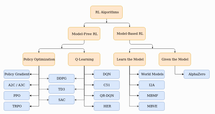Fig 1: Spinningup’s Taxonomy Tree

Materials

This blog post was based in a lot of available material online. We strongly encourage checking out these materials after reading this post for a better understanding of these topics:

• PPO Paper: Paper that proposed PPO in 2017.
• SAC Paper: Paper that proposed PPO in 2019.
• Spinningup RL Algorithms Taxonomy: Spinningup provides simple documentation of the key concepts of RL algorithms.
• Stable Baselines’ RL Resources: A slightly more up-to-date RL resource list provided by Stable Baselines.
• Lillian Weng’s Blog: Lillian Weng is an Open AI researcher that frequently post content about Machine Learning and Reinforcement Learning. This post covers RL algorithms that use Policy Gradients, which includes PPO and SAC.

Background

In this section will remember important RL concepts such as:

• RL Objective
• RL algorithm basic logic
• Monte Carlo Estimation
• Bootstrapping/Bellman Backup

These are the RL topics we think are crucial to understand the basic workings of SAC and PPO and properly compared them. Additional information about some of these topics can be found in an earlier post.

Reinforcement Learning Objective

The Reinforcement Learning paradigm can be formulated as an optimization problem. These class of algorithms normally optimizes the $J(\theta)$ function, expressed in Eq. \eqref{eq:rl_objective}. Typically, we have a reward function $r(s_t, a_t)$ that depends on the action $a$ and state $s$ at the timestep $t$. This reward function is summed over a sequence of timesteps to get the cumulative reward. Finally, the definition of $J(\theta)$ becomes the expected value of the cumulative reward over trajectories created by our RL agent ($\theta$ is the weight vector that parameterizes the agent).

\[\begin{equation} J(\theta)= E_{\tau\sim p_\theta(\tau)}[\sum_t r(s_t,a_t)] \label{eq:rl_objective} \end{equation}\]

Normally, RL algorithms that do Policy Optimization use gradient ascent in this objective function, as expressed in Eq \eqref{eq:rl_objective_gr}.

\[\begin{equation} \theta^*=arg \max_\theta J(\theta) \label{eq:rl_objective_gr} \end{equation}\]

To apply gradient ascent, we differentiate the J(θ) function with respect the parameters θ. Jumping through all the derivation (Spinningup’s derivation), we get that the gradient of the objective function can be estimated according to Eq \eqref{eq:rl_objective_gr_app}.

\[\begin{equation} \nabla J(\theta) \approx \frac{1}{N}\sum_{i=1}^N\sum_{t=1}^T\nabla_\theta \log\pi_\theta(a_t|s_t)(\sum_{t'=t}^Tr(s_{t'},a_{t'})) \label{eq:rl_objective_gr_app} \end{equation}\]

In Eq \eqref{eq:rl_objective_gr_app}, the expectation was replaced by the averaged outcome over $N$ trajectories, and that’s why we now utilize the approximation sign. Inside that sum, the gradients are calculated multiplying the gradient of logarithm of the policy $\nabla_\theta\log\pi_\theta(a_t|s_t)$ and the cumulative reward $\sum_{t’=t}^Tr(s_{t’},a_{t’})$. This second term is also called the Q-function, and will be useful in Actor-Critic implementations.

Reinforcement Learning Algorithms Structure

For almost the entire class of RL algorithms (including actor-critic), the algorithm architecture follows the diagram in figure 2. The process is cyclical, and has three distinct phases. There is a data acquisition phase (orange box), where our agent interacts with the environment and records the states seen, action taken and rewards received. Utilizing this data, we can estimate the cumulative rewards (also called Returns), utilizing a variety of methods (green box). Finally, utilizing the evaluation performed in the green stage, we can improve the policy (blue box). Normally, in Policy Gradients and Actor-Critic methods, the policy is improved directly using gradient ascent.

Fig 2: Basic logic of RL algorithms

Normally, the difference between RL algorithms are found in the way we accomplish the stage green and blue. For example, in the returns’ estimation, Actor-Critic algorithms inspired by Q-learning normally use bootstrapping/Bellman Backup, whereas other algorithms calculate the returns using Monte Carlo estimation.

Monte Carlo Estimation

Monte Carlo estimation involves estimating the value of a state or state-action pair by averaging the returns $G_t$ obtained from sampled episodes, as expressed in Eq \eqref{eq:return}. The

\[\begin{equation} G_t=r_t+\gamma r_{t+1}+\gamma^2 r_{t+2}+\gamma^3 r_{t+3} \dots \label{eq:return} \end{equation}\]

The expectation of the return $G_t$ is called the value function and it is defined in Eq \eqref{eq:value_f}.

\[\begin{equation} V^\pi(s)=\mathbb{E}_{T\sim\pi}[G_t|s_t=s] \label{eq:value_f} \end{equation}\]

This Value function $V^\pi(s)$ will be important later when we talk about PPO. This function tells us how good it is to be in a particular state, accounting for will happen in the future states. In this method, we are always calculating the real return $G_t$, and using that information to update our knowledge of $V^\pi(s)$, however, we need to wait until the end of the episode to update it. The Monte Carlo estimator also is known to have a higher variance, usually needing more data points to get a useful estimation. Despite that, the estimator is unbiased, meaning that with infinite data it will converge to the true value.

Bootstrapping/Bellman Backup

The term Bootstrapping in the context of reinforcement learning and the Bellman backup refers to the idea of pulling oneself up by one’s bootstraps, an expression that means relying on one’s own efforts and resources to achieve something. In the context of reinforcement learning, bootstrapping refers to the use of current value estimates to update and improve those very estimates.

Eq \eqref{eq:q_function} shows the Bellman Backup operation using the Q-function, although it could be used in the Value function $V^\pi(s)$. We choose to show it with the Q-function because it will be important later for SAC. Analyzing Eq \eqref{eq:q_function}, it is apparent the Bootstrapping nature of the estimator, because we use previous knowledge of the Q-function to update itself.

\[\begin{equation} Q(s,a)\leftarrow r(s,a)+\gamma \max_aQ(s,a) \label{eq:q_function} \end{equation}\]

In contrast with Monte Carlo, the Bellman Backup updates the knowledge about the value function at each data point collection, and does not need to wait for the end of the episode. Additionally, this estimator has less variance, needing fewer data points to converge. However, this estimator is biased, meaning that it might converge to a value slightly deviated from the true value.

Soft Actor-Critic

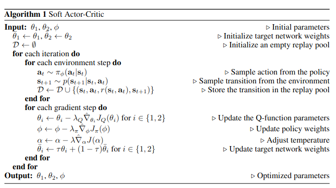Fig 3: SAC Neural Networks architecture (without target network) & pseudo algorithm from the original paper

SAC is an Actor-Critic algorithm that uses the two separated neural networks for the actor (policy) and the critic (Q-function), as shown in figure 3. SAC incorporates the entropy measure of the policy into the reward to encourage exploration, altering the original $J(\theta)$, as shown in Eq \eqref{eq:sac}. This results in a policy that acts as randomly as possible while it is still able to succeed at the task.

\[\begin{equation} J(\theta)= E_{\tau\sim p_\theta(\tau)}[\sum_t r(s_t,a_t) + \alpha\mathcal{H}(\pi_\theta( . | s_t))] \label{eq:sac} \end{equation}\]

To optimize this objective, the author proposed a loss function to minimize for each neural network. Firstly, they proposed $L_1$ in Eq \eqref{eq:sac_loss}, which updates the policy network. Intuitively the way to minimize this function is to minimize $\log\pi$ (actions taken become less probable, therefore we explore actions not taken) or to increase the Q-function (higher Q-function means that we are solving the task). They also prove that updating the policy weights to minimize this loss maximizes the RL objective.

\[\begin{equation} L_1 = J_\pi(\phi)= E_{s_t\sim\mathcal{D}}[E_{a_t\sim\pi_\phi}[\alpha\log(\pi(a_t|s_t)) - Q_\theta(s_t, a_t)]] \label{eq:sac_loss} \end{equation}\]

Secondly, to learn the Q-function network, the authors utilize a Soft Q-learning method. This method is basically the Bellman Backup with an additional entropy term, as shown in Eq \eqref{eq:sac_ent}. Therefore, the second loss ($L_2 = J_Q(\theta)$) is the Mean Squared Error between the left and right side of Eq \eqref{eq:sac_ent}. The entropy component results in adding a bonus reward to actions with less probability.

\[\begin{equation} Q(s_t,a_t)\leftarrow r(s_t,a_t)+\gamma Q(s_{t+1},a_{t+1}) - \alpha\log\pi(a_{t+1} | s_{t+1}) \label{eq:sac_ent} \end{equation}\]

Another interesting property of SAC is its off-policy nature. In figure 4, we can see two for loops for each iteration: the data gathering loop and the gradient step loop. In the first one, the agent is just interacting with the environment and storing the data in the buffer $\mathcal{D}$. In the gradient step loop, the algorithm samples mini-batches from the buffer to calculate the losses and update the neural networks. This means that we are updating our policy with data that was collected by an old policy, making it an off-policy method. Off-policy methods tend to be more unstable, however, its data efficiency and Q-learning style value estimation makes SAC a good candidate to train robotic agents (even in real life). Additionally, there is no practical difference between a dynamic buffer and a static dataset, so SAC like algorithms have seen some experimentation for Offline Reinforcement, which show good results in real world robotic tasks.

Proximal Policy Optimization

PPO addresses the challenges of stability and sample efficiency in policy optimization by introducing a clipped surrogate objective function, as shown in Eq \eqref{eq:clip_surr}. This function prevents large policy updates by clipping $1-\epsilon < r_t(\theta) < 1+\epsilon$, promoting more stable training. This $r_t(\theta)$, which is the coefficient between the policy and the old policy, comes from importance sampling. The importance sampling trick basically updates values collected by old policies to match what we would have got if we had used the current policy. This means that we can do multiple updates on the same batch of data and remain on-policy.

\[\begin{equation} L^{CPI}(\theta)= \mathbb{E}[\frac{\pi_\theta(a_t|s_t)}{\pi_{\theta_{old}}(a_t|s_t)}\hat{A}_t]= \mathbb{E}[r_t(\theta)\hat{A}_t] \label{eq:clip_surr} \end{equation}\]

The other component of the surrogate loss is the Generalized Advantage Estimator (GAE) $\hat{A}_t$, Eq \eqref{eq:gae},which is calculated using the Value function. GAE computes the advantage function interpolating the Monte Carlo and Bellman Backup approximation. We can tune this interpolation by using the hyperparameter $\lambda$, where $\lambda=0$ is the same as a Bellman Backup and $\lambda=1$ is the same as Monte Carlo. The normal value for $\lambda$ is 0.9, meaning that it approximates more the Monte Carlo estimation.

\[\begin{equation} \begin{gathered} \hat{A}_t = \delta_t + (\gamma\lambda)\delta_{t+1} + (\gamma\lambda)^2\delta_{t+2} + \dots + (\gamma\lambda)^{T-t+1}\delta_{T-1}, \\ \delta_t= r_t+\gamma V(s_{t+1}) - V(s_t) \end{gathered} \label{eq:gae} \end{equation}\]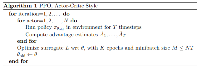

Fig 4: Pseudo algorithm from the original paper

Fig 5: SAC Neural Networks architecture (without target network)

PPO is an Actor-Critic algorithm that uses a single neural network with two heads: one for the actor (policy) and another for the critic (Value function), as shown in figure 5. This neural network is optimized by minimizing a loss function with 3 components, where the surrogate loss is one of them. Eq \eqref{eq:loss_surr} defines the loss $L$ used in PPO.

\[\begin{equation} \begin{gathered} L = L^{CLIP} - c_1L^{VF}+c_2\mathcal{H}(\pi_\theta( . | s_t)), \\ L^{CLIP} = \min(r_t(\theta)\hat{A}_t,\text{clip}(r_t(\theta), 1-\epsilon, 1+\epsilon)\hat{A}_t), \\ L^{VF} = (V_\theta(s_t) - V_t^{\text{targ}})^2 \end{gathered} \label{eq:loss_surr} \end{equation}\]

The third component of the loss function is the entropy of the policy, that incentivizes exploration. By default, this component is not used because $c_2$ is set to zero.

Figure 4 shows the pseudocode of PPO. In contract with SAC, there is no replay buffer. Instead, for each iteration we run the policy for $T$ timesteps in the environment and store the data. After that, use the data as a dataset, and perform $K$ train epochs dividing the data into $M$ sized mini-batchs.All of these values become hyperparameters that need to be carefully tuned when using this algorithm.

SAC vs PPO: Comparison

Now that we have analyzed how each the algorithms works, we will compare some relevant properties of these two algorithms. These properties are exposed and compared in following table. As we can see, both algorithms have their pros and cons, and must be tested in each use case to access which of them is better suited.

Aspect	SAC (Soft Actor-Critic)	PPO (Proximal Policy Optimization)
Algorithm Type	Off-policy	On-policy
Policy Updates	Optimizes policy and Q-function	Focuses on optimizing policy
Exploration Strategy	Entropy regularization for exploration	Balances exploration and exploitation
Policy Representation	Typically stochastic policy	Can be used with stochastic or deterministic policies
Markov Assumption	Strong Markov Assumption (because of Bellman)	Weaker Markov Assumption (because of Monte Carlo)
Bias of Estimators	May have bias due to off-policy learning	Can have low bias due to on-policy learning
Variance of Estimators	Lower variance compared to on-policy methods	May have higher variance, especially in high-dimensional action spaces
Batch vs. Online Learning	More suitable for batch learning with replay buffer	Designed for online learning without relying on a replay buffer
Sample Efficiency	More sample-efficient due to replay buffer	May require more samples from the environment
Application Domains	Commonly used in continuous control and robotics	Widely used in various reinforcement learning tasks
Update Mechanism	Actor-critic with entropy regularization	Clipped surrogate objective for stability
Hyperparameters to optimize	Fewer hyperparameters and less sensible to hyperparameter variation	More hyperparameters and more sensible to hyperparameter variation