Exploding Gradients in Soft-Actor Critic

Introduction

When working with reinforcement learning algorithms, stability and consistency are crucial for achieving optimal performance. One powerful method, Soft Actor-Critic (SAC), combines the benefits of both off-policy learning and entropy regularization to create an efficient, exploration-friendly framework. However, practitioners sometimes face perplexing issues during training, such as exploding gradients. These anomalies can significantly disrupt the learning process, particularly in environments with high-dimensional action spaces.

In this blog post, we will delve into the nuances of this problem, exploring the reasons behind rapidly increasing gradients in SAC and their impact on training. Our exploration will focus on hyperparameter optimization to address this issue. After presenting our results, we’ll discuss possible root causes and identify the most suitable ranges of hyperparameters for this particular experiment.

Experiment Description

Our experiments were conducted in the Gymnasium environment Adroit Relocate. Although the provided documentation is extensive, we’ll summarize key points relevant to our studies, where the problem of exploding gradients emerged due to the environment’s complex action space.

• Learning Objective: An anthropomorphic hand, based on the real Shadow Hand, needs to pick up a ball from a random position and move it to a randomly generated target position.
• Degrees of Freedom: The hand has 30 degrees of freedom — 6 for the arm position and 24 for the hand joints (2 for the wrist, 4 for each finger, and 5 for the thumb). These degrees of freedom constitute the action space.
• Observation Space: The observation space has 39 dimensions, comprising the action space’s 30 dimensions and 3 Cartesian space differences (palm to ball, palm to target, and ball to target).
• Reward Function: The reward function includes a constant component — the negative distance between the palm and the ball. An additional component is added when the ball is lifted beyond a threshold, penalizing the distance between the ball and the target. Finally, if the ball is very close to the target, the agent receives a bonus reward.

Optimization Description

As previously mentioned, there are many causes for exploding gradients in deep learning, and identifying these causes is not always straightforward. To address this, we conducted an intensive hyperparameter optimization to discover the experimental setup that provided the most stability for SAC in this environment and to understand why our experiments consistently experienced exploding gradients.

Although we tried some gradient normalization techniques, we excluded others to reduce the search space for the optimization algorithm. The excluded techniques were normalizing inputs, outputs, and reward function and batch normalization. We opted not to use these techniques because the inputs, outputs, and reward function in the pre-made environment did not reach large values during training, with none exceeding an absolute value of 3. Batch normalization, typically recommended for deeper networks, addresses normalizing values within the network.

The monitored quantity for this optimization procedure was the critic’s maximum achieved gradients during the full training process. The goal of the optimization was to minimize this maximum gradient and identify hyperparameters that could produce controlled learning in a high-dimensional action space environment.

To further reduce the search space, we used discretized educated guesses. We employed Bayesian optimization through Wandb, which leverages knowledge from previous data points (i.e., runs) to make informed guesses for subsequent hyperparameter trials. For context, there were 2,700 possible hyperparameter combinations, and the optimization algorithm only experimented with 210 runs, corresponding to 135 days of compute time (7 days when parallelized). Each training run was set to last 1,500,000 environment steps, and with an average training speed of 25 fps, this translated roughly to 16 hours of training per trial. An exception was made for early stopping if the critic’s gradients exceeded a threshold of 5,000, which we arbitrarily chose as a point of no return based on previous experiment.

Hyperparameters

For the optimization, we focused on a search space that controlled aspects potentially influencing gradients:

Hyperparameter	Description	Search Values
Batch Size	Number of samples seen for each gradient step. Larger batch sizes tend to average out outliers and smoothing out the training. process.	[128, 256, 512]
Entropy Coefficient	SAC includes an exploration bonus component added to the reward function, represented by the symmetric logarithm of the chosen action’s probability. The entropy coefficient scales this bonus component.	[0.00001, 0.0001, 0.001, 0.1, 1]
Gradient Norm Clipping	This technique involves normalizing the norm of the gradient vector, scaling down gradient values while maintaining the correct learning direction. Gradient norm clipping sets a maximum norm allowed during training before updating the networks.	[0.001, 0.01, 0.1, 1, 10]
Learning Rate	This number multiplies with the gradients in the weight update process, effectively scaling the step taken toward improvement.	[0.000003, 0.00003, 0.0003]
Weight Decay	Large gradients can be traced to large weight values. Weight decay penalizes the network for acquiring large weights by adding the norm of the weights to the network’s loss, effectively reducing weight values to lower the loss function. The weight decay hyperparameter scales this loss component.	[0.00001, 0.0001, 0.001, 0.1]
Network Architecture	The network architecture can influence gradient stability. Generally, larger networks cause more instability. In this case, it was used only fully connected layers with ReLu activations in between.	[[256, 256], [512, 256, 256], [1024, 512, 256, 256]]

Results

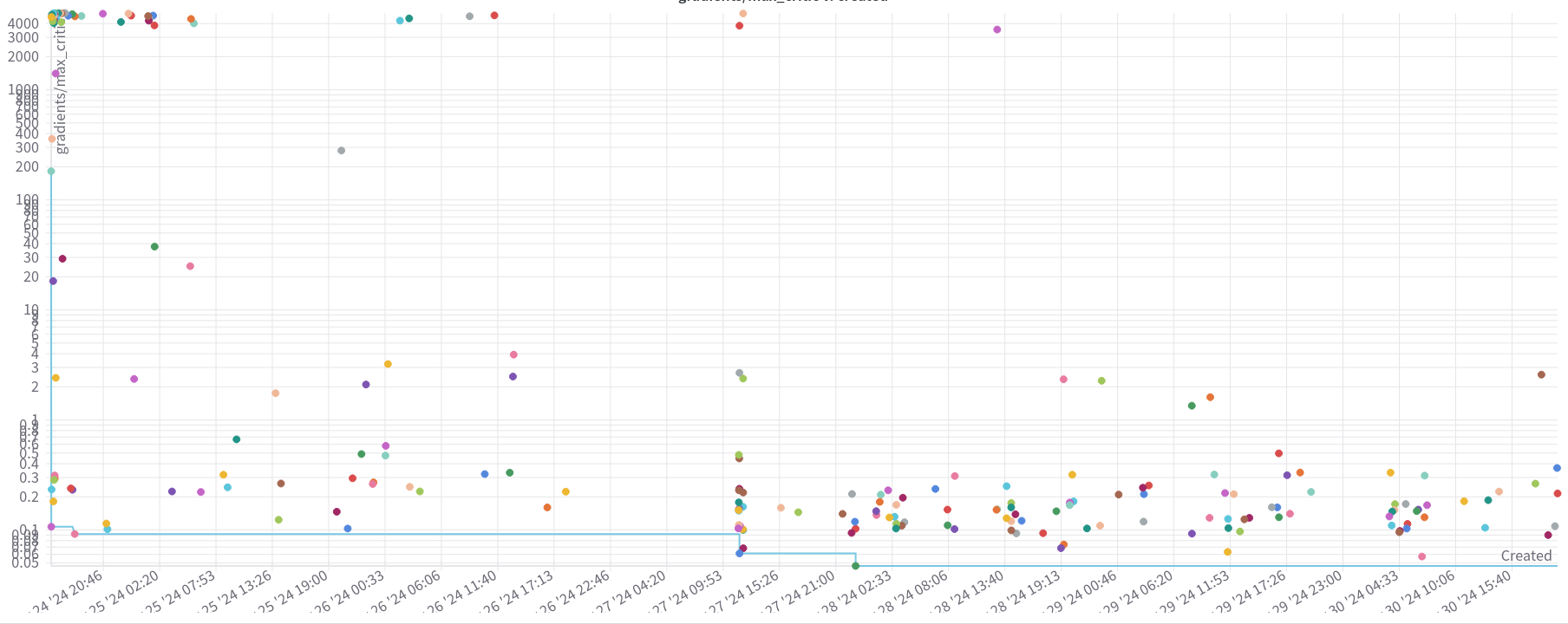
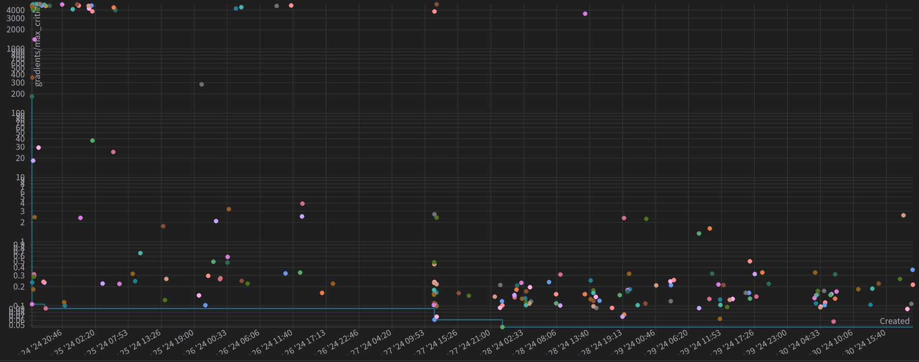Figure 1: Scatter plot for each trial. The y-axis is log-scaled and shows the maximum critic’s gradient achieved. The x-axis represents the date and time when the trial started.

As we can see by the scatter plot, a lot of the first trials exploded the gradients, as we see a concentration of points in the left upper corner. However, along the time axis, we can see that the scatter plots starts to concentrate more in the lowers gradients. We can then postulate that the optimization algorithm learned to propose hyperparameters that maintained stable run, and the results of the optimization process can be trusted.

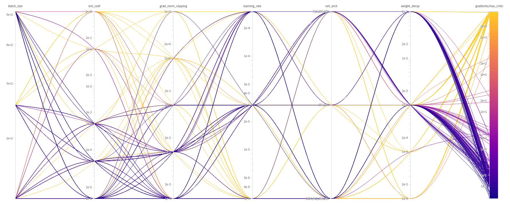
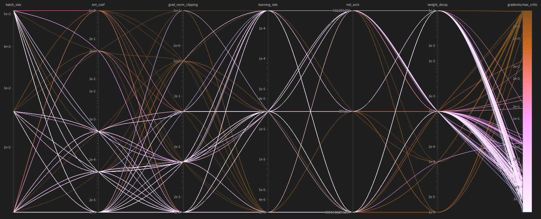Figure 2: Diagram correlating the hyperparameters used with the maximum critic’s gradients achieved. Color coding is utilized to easily visualize which hyperparameters consistently resulted in high or low gradients and which were less relevant. The maximum gradient’s bar is log-scaled.

The diagram offers a qualitative view of the hyperparameters’ importance. For instance, the color concentrations indicate that lower values of maximum critic’s gradients are produced by higher weight decays, lower gradient clippings, and lower entropy coefficients. The one-sided distribution of these parameters suggests they are the most influential. In contrast, hyperparameters like learning rate, network architecture, and batch size exhibit a more spread-out distribution in the maximum critic’s gradients, likely due to their lesser influence.

These qualitative observations can be verified in the following table of correlations and importance weights.

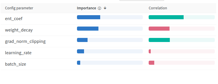
Figure 3: Table presenting the importance weight and correlation between the numeric hyperparameters and the maximum critic’s gradient.

The table shows that the entropy coefficient, weight decay, and gradient clipping are the most effective hyperparameters for preventing gradient explosion.

Entropy Coefficient

The entropy coefficient scales down the exploration bonus inherent to SAC. This entropy bonus is defined by the expected value of the negative logarithm of the probability of an event \eqref{eq:entropy}, in this case, the action taken. In SAC, the policy does not output a specific action but rather a Gaussian distribution of actions by providing a mean and a variance. While not straightforward, it can be assumed that smaller variances result in smaller exploration bonuses, while larger variances result in larger exploration bonuses. This concept is related to Optimistic Exploration. When the agent provides a larger variance, it indicates uncertainty about the best action. In Optimistic Exploration, unknown actions are treated as potentially good actions, hence the bonus. If the action turns out to be suboptimal, the agent learns from the experience.

\[\begin{equation} H(X)=\mathbb{E}[-\log p(X)] \label{eq:entropy} \end{equation}\]

Figure 4 illustrates an example of this concept, showing the logarithm of the probability of actions taken throughout a trial run where gradients exploded. Such plots can be observed in both exploded and non-exploded scenarios. It is possible that larger values, when added to the reward function, create instability in the gradients. This may explain why smaller values of the entropy coefficient contribute to greater stability, as they add smaller components to the reward, keeping it within more stable ranges.

For example, an entropy coefficient of $0.1$ would add to the reward values between $10$ and $30$, where the reward is supposed to be between $−1$ and $1$. These differences in scale could easily create instability in the networks and produce larger and larger gradients.

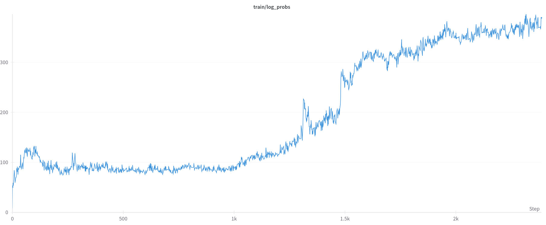
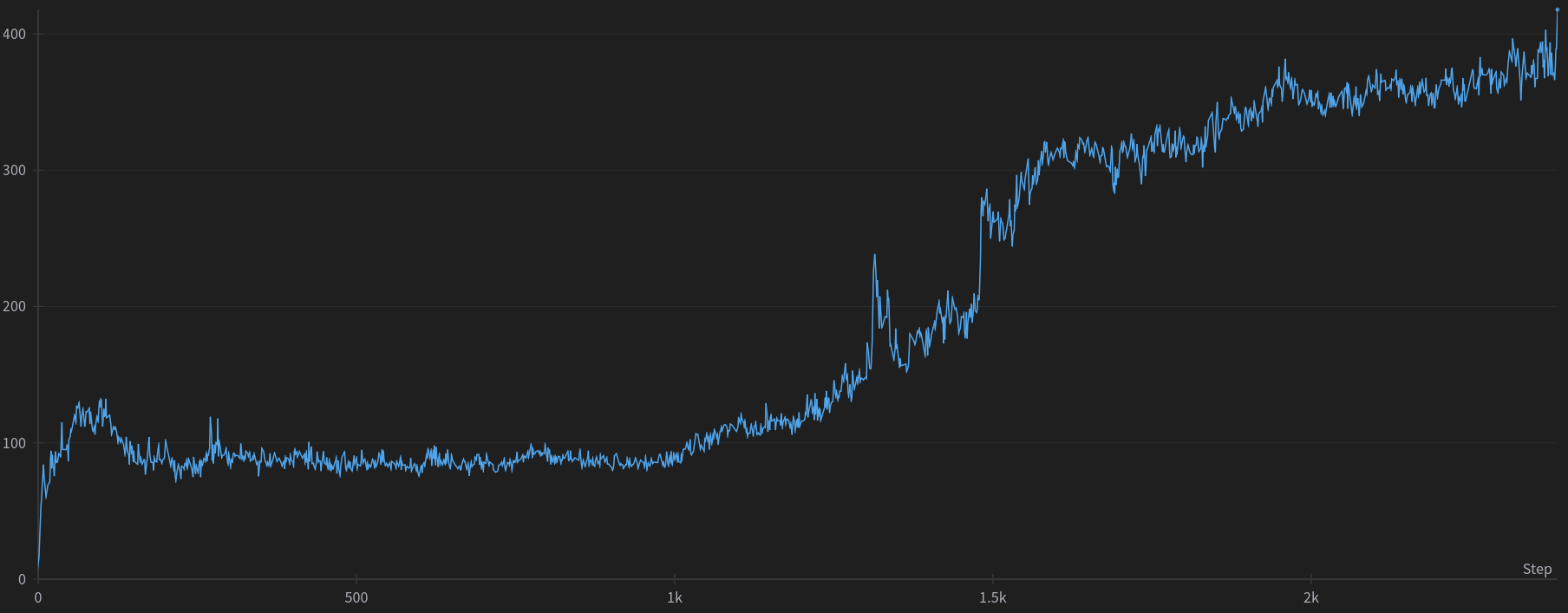Figure 4: Logarithm probability of random trial.

Weight Decay

Intuitively, weight decay continuously applies a “brake” to the growth of the weights. This braking effect prevents any runaway growth that could lead to exploding gradients. By keeping the weights smaller, the gradient magnitudes also tend to be smaller, since the gradients are often proportional to the weights. Smaller gradients mean less drastic updates, reducing the chance of gradients exploding.

This effect is evident in the optimization results, which show a negative (red) correlation between the value of the gradients and the weight decay hyperparameter. As previously mentioned, the weight decay parameter scales the penalization of the weight’s norm, meaning higher weight decay penalizes the weights more, resulting in smaller valued weights and, theoretically, smaller gradients. This theory was validated in the optimization setup.

Furthermore, weight decay, being a regularization technique, is typically used to avoid overfitting. This provides an interesting insight: if our agent overfits to a specific area of the state-action space, any change in state or action might produce unpredictable outputs, leading to huge losses and, consequently, huge gradients. Thus, avoiding overfitting may indirectly prevent exploding gradients.

Regardless of the interpretation, it is clear that weight decay is crucial for a well-behaved training session and should be set to a significant value.

Gradient Clipping

Gradient clipping, while not as crucial as the other two hyperparameters, still plays an important role in preventing gradient explosions and shows a high correlation with gradient stability. Gradient clipping is straightforward: it limits the size of gradients and the step taken during optimization. However, as shown in previous experiments, the instability might be causing the gradient explosion, rather than being caused by it. Therefore, clipping the gradients might only address the symptom of the problem, not the root cause. This might explain why gradient clipping is not as effective as other methods. It helps contain the problem but does not resolve it.

The gradient clipping threshold has a positive (green) correlation with the magnitude of the gradients. This means that to lower the gradients, we need to lower the clipping threshold.

Suggested Hyperparameters

The following diagram highlights the hyperparameters used in the various runs the achieved maximum gradient norm of $1$ or less.

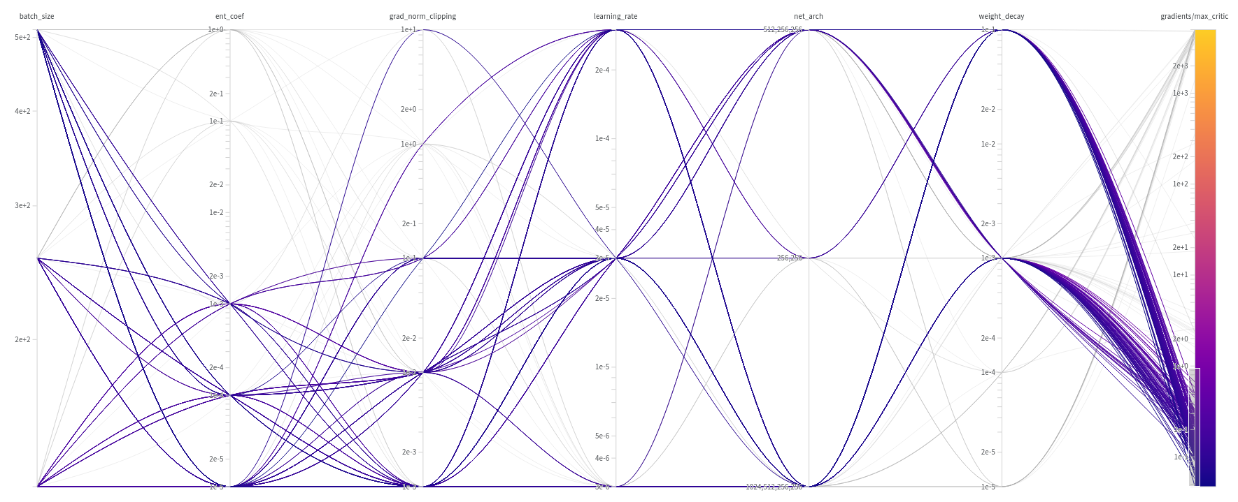
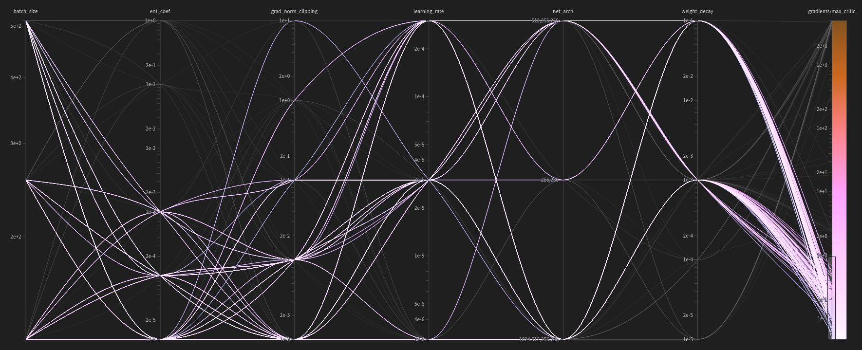Figure 5: A diagram correlating the hyperparameters used with the maximum critic’s gradients achieved. In this diagram, the trials that obtained maximum gradients less than $1$ are highlighted.

Based on this diagram, we can propose a list of hyperparameters that should be used to maintain controlled gradients:

• Batch Size: $[128, 256, 512]$
• Entropy Coefficient: $[0.001, 0.0001, 0.00001]$
• Gradient Norm Clipping: $[0.1, 0.01, 0.001]$
• Learning Rate: $[0.000003, 0.00003, 0.0003]$
• Weight Decay: $[0.1, 0.001]$

The network architecture does not seem to be relevant in this study, given the widely varying gradient values it produces. This is advantageous as it allows for flexibility in the size of networks we use.

Problem: Not Learning

One crucial issue that hasn’t been addressed yet in this post but has been a persistent concern during our experiments is: what happens to the learning process if we minimize the gradients too much? Minimizing the gradients excessively can halt the learning process altogether. Gradients provide the direction and step size necessary for optimizing our network to produce the desired output for a given task. If the gradients become too small, there’s a risk that the network will not be updated sufficiently, resulting in minimal or no meaningful changes during training.

This phenomenon is illustrated in Figure 6, which shows the plot of the average cumulative reward per episode throughout the trial that achieved the lowest maximum critic gradients ($0.047$). As depicted, the reward fails to improve, consistently remaining around $-1$.

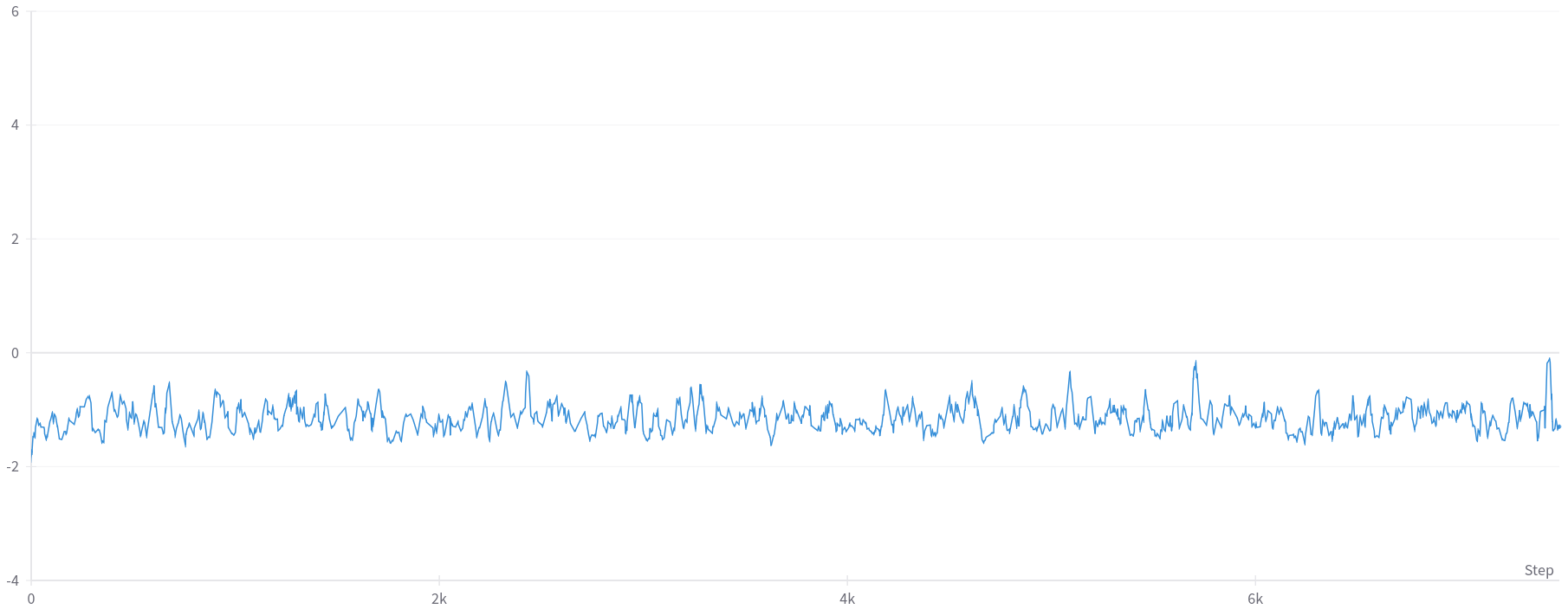
Figure 6: Plot of the cumulative episode reward throughout the trail with the lowest maximum critic’s gradients ($0.047$).

On the contrary, in Figure 7, we observe a trial with controlled maximum critic gradients ($2.58$), significantly higher in magnitude compared to the lowest obtained through the optimization method. Despite this trial’s failure to effectively solve the environment (as evidenced by a zero success rate), there’s a notable observation: the agent is indeed learning and adapting its behavior throughout the training process without encountering instability.

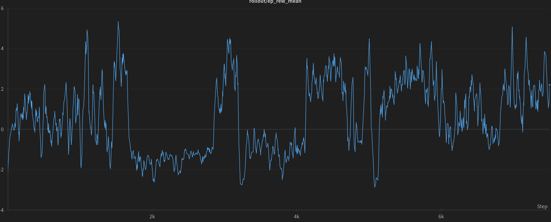Figure 7: Plot of the cumulative episode reward throughout the trail with controlled maximum critic’s gradients ($2.58$).

Dark mode might be best to visualize the following graphs/diagrams

Taking a broader perspective, we can manipulate the visualization to emphasize trials that attained a reward greater than $0$, as illustrated in Figure 8. It’s worth noting that the y-axis of the scatter plot is displayed on a logarithmic scale. Contrary to expectations, the trials achieving a positive reward were not characterized by lower gradients. Intriguingly, upon excluding the outliers, it becomes apparent that they consistently reach the same maximum gradients.

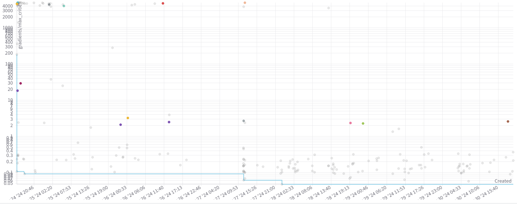
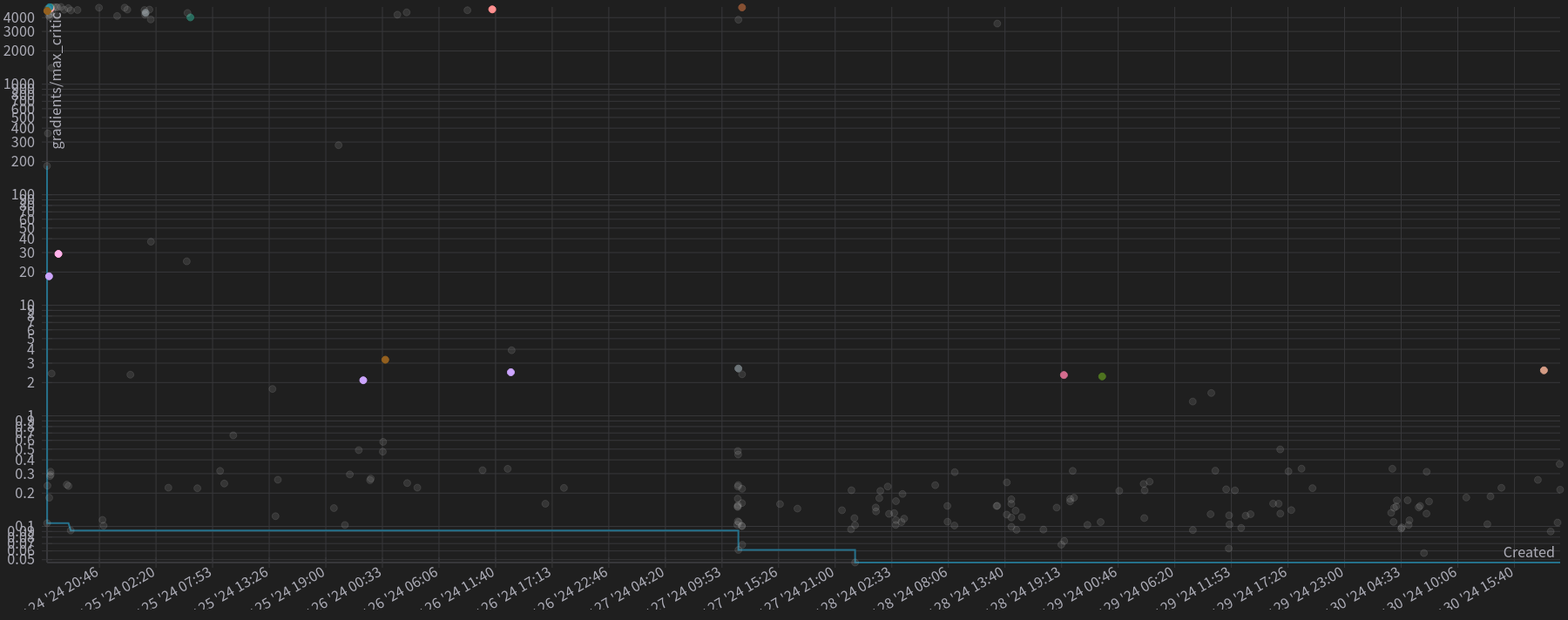Figure 8: Scatter plot for each trial. The y-axis is log-scaled and shows the maximum critic’s gradient achieved. The x-axis represents the date and time when the trial started. The dots highlighted represent the trails that achieved final mean episodic reward greater than $0$

Additionally, we can manipulate the visualization of the hyperparameter diagram to establish a relationship between the hyperparameters and the reward. Figure 9 presents a diagram that correlates the hyperparameters of a trial with the final mean episodic reward, specifically highlighting the trials that achieved a reward greater than $0$.

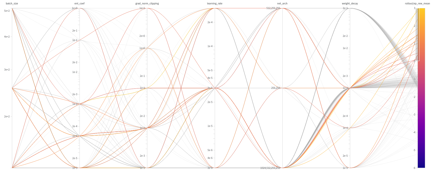
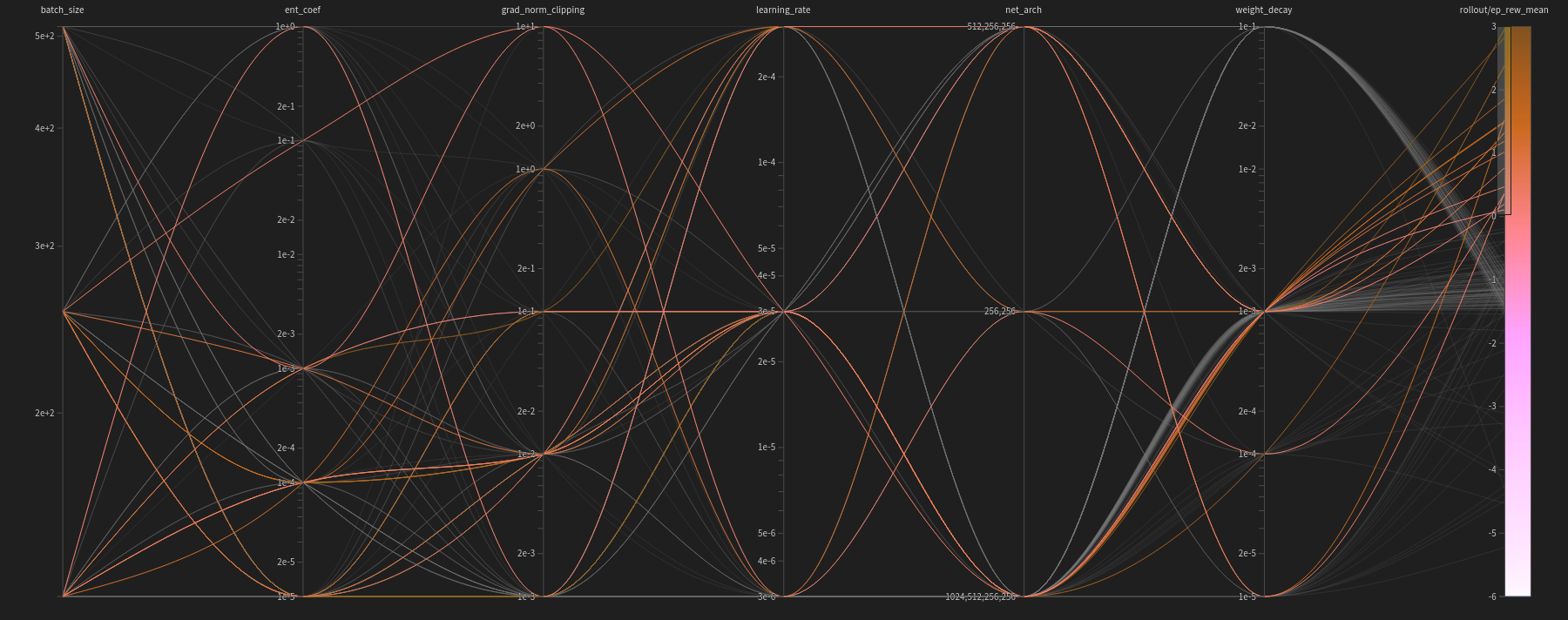Figure 9: A diagram correlating the hyperparameters used with final mean episodic rewards achieved. In this diagram, the trials that obtained rewards greater than $0$ are highlighted.

Upon analyzing this diagram, it becomes evident that for the agent to exhibit some degree of learning (i.e., achieving a reward greater than $0$), the following hyperparameters are recommended:

• Batch Size: $[128, 256, 512]$
• Entropy Coefficient: $[0.001, 0.0001, 0.00001]$
• Gradient Norm Clipping: $[0.001, 0.01, 0.1, 1, 10]$
• Learning Rate: $[0.000003, 0.00003, 0.0003]$
• Weight Decay: $[0.00001, 0.0001, 0.001]$

Comparing these hyperparameters to those obtained by purely minimizing the gradients, the most notable difference lies in the weight decay parameter. In this scenario, the highest weight decay, which was favored previously, is not permitted. This observation aligns with expectations because an excessive penalty on the weights’ magnitude, instead of solely preventing overfitting, typically obstructs learning altogether. Such stringent weight constraints restrict the weights’ flexibility to adjust to the values required for effective learning.

By taking the intersection of the hyperparameters from the list provided earlier, we can identify choices that simultaneously avoid exploding gradients while enabling the agent to learn. These optimal hyperparameters would be:

• Batch Size: $[128, 256, 512]$
• Entropy Coefficient: $[0.001, 0.0001, 0.00001]$
• Gradient Norm Clipping: $[0.001, 0.01, 0.1]$
• Learning Rate: $[0.000003, 0.00003, 0.0003]$
• Weight Decay: $[0.001]$

Conclusion

In conclusion, this optimization procedure has significantly enhanced our understanding of the stability challenges encountered in training SAC and neural networks in general. It has shed light on the influence of various hyperparameters on gradient behavior. We believe we have arrived at a satisfactory conclusion and identified a set of hyperparameters for future research endeavors.

Moving forward, our next step is to implement these hyperparameters in training setups aimed at solving the specific task, with the assurance that stability during training is effectively addressed.

As a documented proposal, we recommend the adoption of the following set of hyperparameters going forward:

• Batch Size: $256$
• Entropy Coefficient: $0.0001$
• Gradient Norm Clipping: $0.01$
• Learning Rate: $0.00003$
• Weight Decay: $0.001$