Invicta School: Causality for Machine Learning

This is a summary of Julius von Kügelgen’s presentation titled “Causality for Machine Learning.” In his talk, he explored the mathematical concepts behind causality and how they differ from traditional statistics. He also discussed the importance of a causal framework in machine learning, which typically relies on statistical methods.

The main focus of the presentation was on the theory of causal inference, covering both causal reasoning and causal discovery. It was only towards the end that the presenter mentioned how the challenges or methodologies of causal inference could intersect with machine learning. The discussion on machine learning primarily aimed to inform the audience about existing approaches, obstacles, and potential future directions for integrating causality and machine learning.

In the disclaimers, Dr Kügelgen mentions that this presentation was based on Elements of Causal Inference by Peters et al. (2017), and on From Statistical To Causal Learning by Schölkopf et al. (2022).

This summary will follow the a structure used in the presentation:

• Introduction and Motivation
• Causal Models and Causal Reasoning
• Principle of Independent Causal Mechanisms
• Learning Cause-Effect Models
• Learning Multivariate Causal Models
• Causal Time Series and Granger Causality
• Connections to Machine Learning
• Causal Representation Learning

Introduction and Motivation

Causation definition (Total Causal Effect): X has a (total) causal effect on Y if there are distinct values $x \neq x’$ such that the distribution of Y differs when changing $X$ from $x$ to $x’$.

Causation definition (Total Causal Effect): $X$ has a (total) causal effect on $Y$ if there are distinct values $x\neq x’$ such that the distribution of $Y$ differs when changing $X$ from $x$ to $x’$.

According to Kügelgen’s definition, the study of causation is called Causal Inference (CI), which is subdivided into two groups: Causal Learning (Discovery) and Causal Reasoning. Analogous to traditional Machine Learning, Causal Learning is the process of learning a model through data, and Causal Reasoning is the process of obtaining data through the model, as represented by the following image.

Fig 1: A diagram comparing the similarities between statistical learning (machine learning) and causal inference

The final motivation for causality is that “correlation does not equal causality,” which means that learning models purely on correlation (traditional machine learning) can lead to errors in predictions. An example presented in the presentation was the close correlation between ice cream consumption and the number of drownings, as depicted in the image below.

Does this mean that we should stop eating ice cream before swimming? Or that increased drowning increases the population’s appetite for ice cream? In fact, there is a third confounding variable presented in the graph: the month of the year. The month of the year influences both ice cream consumption and the number of drownings, creating a correlation between them, despite the absence of causal influence between them.

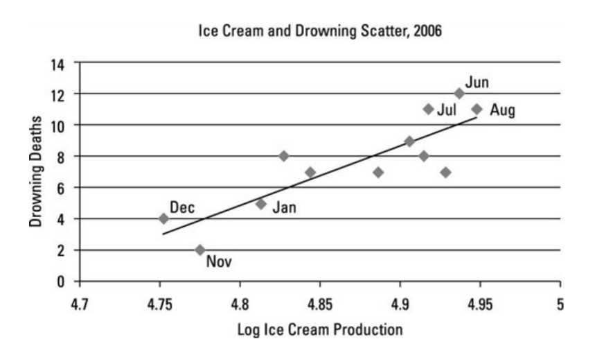Fig 2: A graph that depicts a strong correlation between ice cream consumption and drownings, although they have no causal association

If two random variables X and Y are statistically dependent (\(X \not \perp\!\!\!\!\!\perp Y\)), then there exists a third variable Z that causally influences both (As a special case, Z may coincide with X or Y). Furthermore, this variable Z screens X and Y from each other in the sense that given Z they become independent, \(X \perp\!\!\!\perp Y | Z\)

The common cause principle establishes a link between statistical properties and possible causal structures. This means that, if $X$ and $Y$ are statistical dependent, then the causal structure must be one of the following:

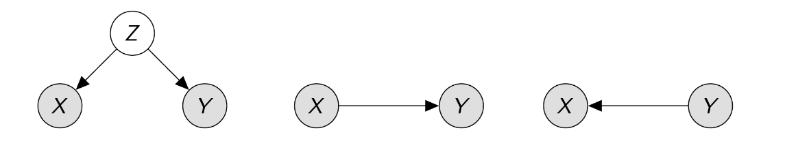Fig 3: The common cause principle establish a link between statistical dependence and one of these causal structures

This implies that while we cannot fully define a causal structure solely based on statistical properties, we can narrow down the possibilities and guide our search for causal relationships.

Causal Models and Causal Reasoning

A Causal Model (e.g. Structure Causal Models) entail:

• Causal Graph
• Observational Distribution
• Intervention Distribution
• Counterfactuals

More informally, while a statistical model can be conceived as a single distribution (observational distribution), a Causal Model can be seen as a collection (family) of distributions related to each other in a structured way, incorporating interventions and counterfactuals. The image by Schölkopf et al., 2021 visually illustrates this concept.

Fig 4: Difference between the distributions modeled by a statistical model and a causal model

Structured Causal Models (SCM)

Markovian SCM definition: A Markovian structural causal model (SCM) $\mathcal{C} = (S, P_N)$ over observables $X = {X_1, \dots, X_n}$ consists of (i) a collection S of structural equations,

\[\begin{equation} X_j := f_j(PA_j, N_j) \text{ for } j = 1, \dots, n \label{eq:scm} \end{equation}\]

where $PA_j \subseteq {X_1, \dots, X_n} \ {X_j}$ are the causal parents (direct causes) of $X_j$; and (ii) a factorizing joint distribution $P_N = P_{N_1} \times \dots \times P_{N_n}$ over jointly independent (“exogenous”) noise variables $N = (N_1, \dots, N_n)$

Note that \(f_j(.)\) is deterministic, which means that all the stochasticity comes from the noise variables.

We show the same example presented in the presentation, in the following figure.

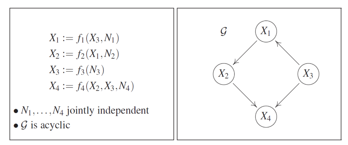Fig 5: Markovian Structural Causal Model

In this example, we have a SCM with 4 variables. The SCM (left) can be partially represented by the causal graph (right) by drawing directed edges from each parent node $PA_j$​ to each $X_j$​. A common assumption is that the causal graph does not contain cycles, i.e., it is a Directed Acyclic Graph (DAG).

With a defined SCM and Causal Graph, if we want to sample an observation, we simply apply ancestral sampling. To sample $X$:

1. Draw $N \sim P_N$
2. Iteratively compute $X_i$​ following the (partial) causal order induced by the graph.

Now we can understand why we assume the SCM creates a DAG. Without the acyclic assumption, we could not sample observations because we could not guarantee that we have a root node to start the sampling process. The acyclic assumption indirectly ensures that there is always at least one root node.

Causal Markov Condition

A SCM associated with a DAG implies the following causal factorization from the observational distribution:

\[\begin{equation} p(X_1, \dots, X_n) = \Pi_{i=1}^n p(X_i|PA_i) \label{eq:scm_condition} \end{equation}\]

where $PA_i={X_j:(X_j \rightarrow X_i) \in G}$ denotes the set of parents, or direct causes, of $X_i$ in $G$. This equivalent to the definition of Causal Markov Condition: a distribution p satisfies the causal Markov condition w.r.t. a DAG G if every variable is conditionally independent of its non-descendants in G given its parents in G.

This Causal Markov Condition is important because it relates the joint distribution over all variables $p$, with a factorization that is more related to a statistical quantity that is more related to a causal quantity.

Hard Interventions and Graph Surgery

It is very useful to reason about interventions in graphs. As depicted by the figure, an intervention transforms the graph G to G’ or G’’ by removing all incoming edges to the intervened variable (diamond). Typically, the intervention is denoted by the do-operator ($do(.)$), which by definition computes a causal quantity (interventions are defined only in causality).

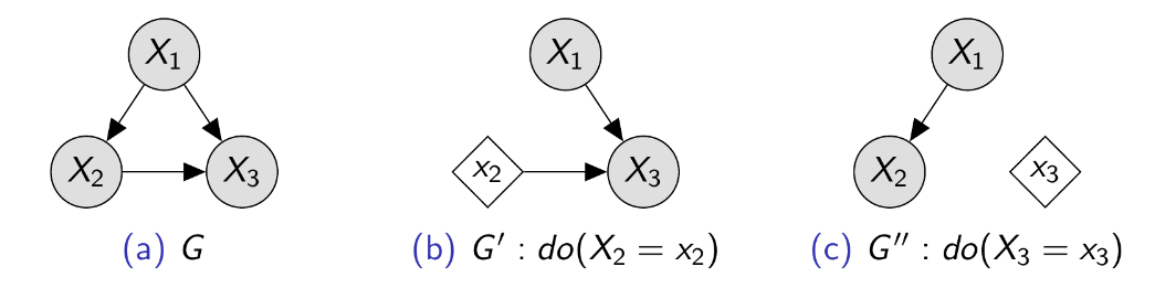Fig 6: Representation of graph transformation when applying hard interventions

This transformation over graphs enables the computation of interventional distributions as conditional distributions, factorized over the corresponding post-intervention graph.

\[\begin{equation} p_G(X_3|do(X_2:=x_2)) = p_{G'}(X_3|X_2=x_2) \rightarrow p(X | do(x_\mathcal{I})) = \mathbb{I}\{X_\mathcal{I}=x_\mathcal{I}\} \Pi_{i\not\in \mathcal{I}} p(X_i|PA_i) \label{eq:hard-inter} \end{equation}\]

This new factorization is commonly referred to as the g-formula, truncated factorization, or manipulation theorem.

The significance of this lies in the fact that, for the first time, we have an equation that links a causal quantity (interventional distribution) with a statistical quantity (conditional probability). This implies that we can “translate” causal quantities into statistical estimands and subsequently utilize traditional statistical methods to compute causal influence.

Simpson’s Paradox

Simpson’s Paradox is a renowned issue in the realm of Causality. Despite being labeled a paradox due to its seemingly contradictory nature, it actually has a logical resolution. Illustrated by the kidney stones example in the table below, the paradox centers on the observation that while treatment B demonstrates superior effectiveness overall, treatment A outperforms in both subgroups when the population is divided based on stone size.

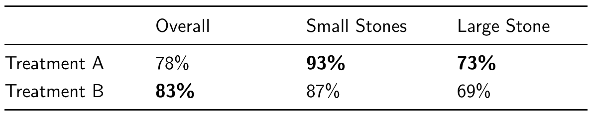Table 1: Percentage of success cases in treating kidney stones

But how can this be? How can treatment A better in both groups, yet treatment B be superior overall? Upon analyzing the new table, which discloses the number of individuals receiving each treatment, we can observe that this is not actually a paradox. What occurred is that, while an equal number of individuals received both treatments, treatment A primarily addressed large stones, whereas treatment B primarily addressed small stones. We can infer that treating small stones inherently carries a higher likelihood of recovery compared to treating large stones, regardless of the treatment administered, and that justifies our findings.

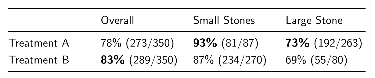Table 2: Percentage of success cases in treating kidney stones and disclosing the absolute values

But is it plausible to find data skewed in this manner? Perhaps the doctors administering the treatments were already aware that treatment A was more effective. Consequently, when a patient presented with large stones, treatment A was recommended. However, treatment B might have been suggested for smaller stones, possibly due to its lower cost or invasiveness. In fact, these are all reasonable assumptions that can occur in the real world, leading to data patterns similar to those observed in this table. In summary, we can observe that the size of the stone (Z) confounds both the treatment (T) and the outcome (Y), as it impacts the treatment choice and the likelihood of recovery. This causal structure is graphically depicted in the following figure.

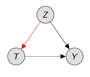Fig 7: Causal graph of the thought experiment showcasing Simpson’s paradox

Computing Counterfactuals with SCM

Interventions are reasoned at a population level, while counterfactuals are reasoned at a individual level.

If we consider a SCM \(\mathcal{M}\) defined by

\[\begin{equation} \begin{aligned} X &:=U_X \\ Y &:=3X+U_Y \\ U_X, U_Y & \sim \mathcal{N}(0, 1) \end{aligned} \label{eq:counter} \end{equation}\]

Suppose that we observe $X=2$ and $Y=6.5$ and to speculate “what would $Y$ haven been, had $X=1$?”

1. Abduction: Update the noise using the observed evidence by plugin in \(X=2\) and $Y=6.5$. We obtain \(U_X=2\) and \(U_Y=0.5\)
2. Action: Performing the intervention \(do(X:=1)\) (replace the structural equation for X)
3. Prediction: computing the push-forward gives the result \(p(Y_{X=1}| X=2, Y=6.5)= \delta(3.5)\), so “Y would have been 3.5”

Note that this is different from the simple intervention \(P(Y|do(X=1)) = \mathcal{N(3,1)}\), since the factual observation helped determine the background state (random variables)

Potential Outcome (PO) Framework

The Potential Outcome Framework offers a different perspective on the causality problem. While SCM and DAG are often more advantageous for Machine Learning implementations, the Potential Outcome Framework provides valuable concepts and definitions for characterizing causal relationships.

Initially proposed by Neyman for randomized studies and subsequently extended to observational settings, the primary concept revolves around viewing causal inference as a missing data problem.

For each individual i and treatment t there exists a PO \(Y_i(t)\) that represents what would happen if individual $i$ received treatment $t$.

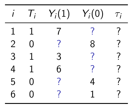Fig 8: Visual represention of the “Fundamental Problem of Causal Inference” as a missing data problem.

1. Individual Treatment Effects The ITE for individual $i$ under a binary treatment is defined as: $\tau_i = Y_i(1) - Y_i(0)$. The ITE measures the complete causal effect between $T$ and $Y$. However, the calculation of the Individual Treatment Effect (ITE) presents a challenge, often referred to as the “Fundamental Problem of Causal Inference”. This problem arises from the fact that for each individual $i$, only one of the POs is observed, while the other becomes a counterfactual. This unobserved counterfactual is the reason why this problem is conceptualized as a “missing data” issue. Just to bridge the PO framework with the theory of SCM,we can consider $Y_i(t)=Y|do(T=t)$
2. Average Treatment Effects The average treatment effect (ATE) is the population average of the of the difference of the outcomes. \(\begin{equation} \tau:=\mathcal{E}[\tau(X)] = \mathcal{E}[Y | do(T=1)] - \mathcal{E}[Y | do(T=0)] = \mathcal{E}[Y(1) - Y(0)] \label{eq:ate} \end{equation}\) The conditional average treatment effect (CATE), is the average difference of the outcomes of a population conditioned on a subset of features. \(\begin{equation} \tau(x):= \mathcal{E}[Y |x, do(T=1)] - \mathcal{E}[Y |x, do(T=0)] = \mathcal{E}[Y(1) - Y(0)| x] \label{eq:cate} \end{equation}\)

Identification in the PO framework

The identification process entails discovering a statistical estimand that corresponds to the estimation of the causal effect. If we can pinpoint such a statistical estimand, we can compute the causal effect using purely observational data. However, to achieve this, we rely on certain assumptions.

1. Overlap/common treatment support: For any treatment t and any configuration of features x, it holds that -> 0 < p(T=t|X=x) < 1 This means that every treatment option as been tested in every possible combination of features at least once.
2. Conditional Ignorability/no hidden confounding: Given a treatment $T \in { 0,1}$, potential outcomes &Y(0)&, &Y(1)&, and observed covariates X, we have \(Y(0) \perp \!\!\! \perp T|X \text{ and } Y(1) \perp \!\!\! \perp T|X\)

With these two assumptions, we ensure identifiability.

In other sources, I have also come across the No Interference and Consistency assumptions, which are more fundamental assumptions and are not explicitly mentioned here. The No Interference assumption posits that the treatment assigned to one individual does not influence the outcomes of other individuals, whereas the Consistency assumption asserts that the observed outcome for an individual under a specific treatment condition is equivalent to their potential outcome under that treatment.

Identification in the Graphical View

Tied to identification in graphical terms is the concept of Valid Adjustment Sets (VAS).

Under causal sufficiency, a set Z is a valid adjustment sets for the causal effet of a singleton treatment T on an outcome Y in the sense of

\[\begin{equation} P(y|do(t)) = \sum_z p(z)p(y|t,z) \label{eq:vas} \end{equation}\]

if and only if the following two conditions hold.

1. Z blocks all non-directed paths from T to Y
2. Z contains no descendant of any node on a directed path from T to Y (except for descendants of T which are not on a directed path from T to Y)

As an example, consider the following graph:

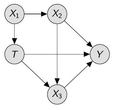Fig 9:Graph example

To block the backdoor paths that connect T and Y (isolating only the effect of the directed paths), the valid adjustments sets are \(\{X_1\}\), \(\{X_2\}\), \(\{X_1, X_2\}\).

We cannot condition on X_3 because it blocks one directed path from T to Y, and it opens the collider path \(T \rightarrow X_3 \leftarrow X_2\)

Average Treatment Effect Estimators

For \(m_1\) observations $(x_i, y_i, t_i = 1)$ from treatment group and $m_0$ observations $(x_i, y_i, t_i = 0)$

RCT estimator (Gold standard; no adjustment necessary):

\[\begin{equation} \hat{\tau}_{RTC} = \frac{1}{m_1}\sum_{i:t_i=1}y_i - \frac{1}{m_0}\sum_{i:t_i=1}y_i \label{eq:rct} \end{equation}\]

Regression adjustment: Fit $\hat{f}$ to $\mathcal{E}[Y | Z = z, T = t]$ where $Z$ is a valid adjustment set; then use $\hat{f}(z, t)$ to impute counterfactual outcomes as $\hat{y}^{CF}_i = \hat{f}(z_i, 1- t_i)$

\[\begin{equation} \hat{\tau}_{reg} = \frac{1}{m_1}\sum_{i:t_i=1}(y_i - \hat{f}(z_i, 0)) + \frac{1}{m_0}\sum_{i:t_i=1}(\hat{f}(z_i, 1) - y_i) \label{eq:adjust} \end{equation}\]

Inverse probability weighting(IPW) estimator (or propensity score)

\[\begin{equation} \hat{\tau}_{IPW} = \frac{1}{m_1}\sum_{i:t_i=1}\frac{y_i}{p(T=1|Z=z_i)} + \frac{1}{m_0}\sum_{i:t_i=1}\frac{y_i}{p(T=0|Z=z_i)} \label{eq:ipw} \end{equation}\]

I think $Z$ still is a valid adjustment set

Nearest Neighbor matching: match and contrast each individual i with the most similar one, $j(i)$, from the opposite treatment group based on $Z$

\[\begin{equation} \hat{\tau}_{NN-matching} = \frac{1}{m_1} \sum_{i:t_i=1}(y_i - y_{j(i)}) + \frac{1}{m_0} \sum_{i:t_i=1}(y_{j(i)} - y_i) \label{eq:NNM} \end{equation}\]

Causal Reasoning with Hidden Confounders/ No overlap

Interventional distributions are not identifiable from observational data when hidden confounders are present or when there is no overlap between treatment groups.

For these cases, we have alternative methods to identify the causal estimand. When we are aware of the confounders, we condition on them, a method known as Backdoor Adjustment. However, in the presence of Hidden Confounders or when there is No overlap, we employ:

1. Front-door Adjustment
2. Instrumental Variable
3. Regression Discontinuity Design

Front-door Adjusment: Use a intermediary variable $M$ which mediates the directed path between $T$ and $Y$. We $M$ must assume that $M$ does not have confounders with $Y$.

\[\begin{equation} p(y|do(t)) = \sum_m p(m|t) \sum_{t'}p(t')p(y|m,t') \label{eq:fda} \end{equation}\]

Instrumental Variable: A variable $I$ is a valid instrumental variable for estimating the effect of treatment $T$ on outcome $Y$ confounded by hidden variable $H$ if all of the following three conditions hold:

1. \[I \perp\!\!\!\perp H\]
2. \[I \not \perp\!\!\!\!\!\perp T\]
3. \[I \perp\!\!\!\perp Y | T\]

In this setup, we begin by regressing $T$ on $I$ to obtain $\hat{T} = aI$. This estimation is no longer dependent on $H$. Consequently, we can then regress $Y$ on $\hat{T}$ to derive the causal effect. If we were to naively regress $Y$ on $T$, it would yield a different confounded result.

Regression Discontinuity Design: Used in scenarios where there is no overlap of values in the VAS, this method involves regressing the values on the treatment group and the control group. Subsequently, we compute the difference where the two meet, as suggested in the following image.

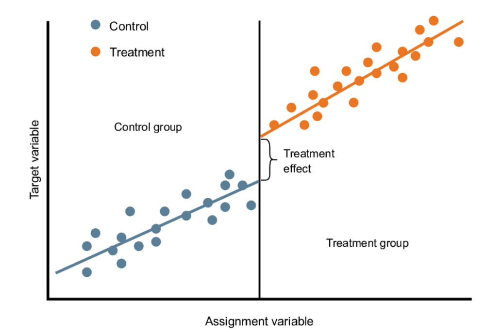Fig 10:Graphical representation of regression discontinuity design

Principle of Independent Causal Mechanisms

To motivate the idea of independent mechanisms, Dr. Kügelgen presents two examples that justify its application:

1. Generic View Point assumption: This assumption posits that the object and the mechanism by which it is perceived are independent. For instance, when observing a chair, the chair remains the same object regardless of changes in viewpoint. Although optical illusions may violate this assumption, they are typically artificially created. Generally, in nature, such violations are either rare or non-existent.
2. Altitude and Temperature example: Consider a joint probability distribution of altitude and temperature, denoted as $p(a,t)$. Statistically, this distribution can be expressed in two ways: $p(a|t)p(t)$ or $p(t|a)p(a)$. However, causally, these two representations are not equivalent. Based on our understanding of the world, altitude influences temperature, rather than the other way around. Thus, the causal mechanism $p(t|a)$ remains invariant to changes in $p(a)$. It represents a physical law that holds true regardless of altitude variations. In statistical terms, knowledge of $p(a)$ does not provide additional information about $p(t|a)$. Conversely, the same principle does not hold for the anti-causal direction, $p(a|t)$, with $p(t)$.

Principle - Independent Mechanisms:

• The causal generative process of system’s variables is composed of autonomous modules that do not inform or influence each other.
• In the probabilistic case, this means that the conditional distribution of each variable given its causes (i.e., its mechanism) does not inform or influence the other conditional distributions.
• In case we have only two variables, this reduces to an independence of cause and mechanism.

My interpretation: Causal mechanisms are conditional probabilities that correspond to physical phenomena.

Learning Cause-Effect Models

The Two variable case

\[\begin{equation} \begin{aligned} C &:= N_C \\ E &:= f_E(C,N_E) \\ N_C &\perp \!\!\! \perp N_E \end{aligned} \label{eq:two_v} \end{equation}\]

It can be demonstrated, through the Common Cause Principle, that statistical information alone is insufficient to determine the causal direction between $C$ and $E$, whether it’s $C \rightarrow E$ or $E \rightarrow C$. Consequently, additional assumptions are necessary. One common approach to address this is by making assumptions about the class of the function $f_E$.

Proposition - Non uniqueness of graph structures: For every joint distribution $P_{X,Y}$ of two real-valued variables,

\[\begin{equation} \begin{aligned} \exists &\text{SCM} \\ X &:=N_X \\ Y &:=f_Y(X,N_y) \\ N_Y &\perp \!\!\! N_X \end{aligned} \label{eq:non_unique} \end{equation}\]

where $f_Y$ is a measurable function and $N_Y$ is a real-valued variable.

The crucial point to grasp from this is that without constraining the function class, both causal directions are feasible.

Disclosure: All of the aforementioned holds true when attempting causal discovery solely with observational data.

Linear Non-Gaussian Acyclic Model (LiNGAM)

Theorem: Identifiability of linear non-Gaussian models

Assume that $P_{X,Y}$ admits the linear model

\[\begin{equation} Y = \alpha X + N_Y \text{, } N_Y \perp \!\!\! \perp X \label{eq:lingam} \end{equation}\]

with continuous $X$, $N_Y$ and $Y$. Then $\exists\beta \in \mathcal{R}$ and $N_X$ s.t.

\[\begin{equation} X=\beta Y + N_X \text{, } N_X \perp \!\!\! \perp Y \label{eq:lingam2} \end{equation}\]

if and only if $N_Y$ and $X$ are Gaussian. This theorem can also be generalized to the multi-variate setting.

Darmois-Skitovich Theorem

For $K \ge 2$ let $Z_1, \dots, Z_k$ be mutually independent, non-degenerate random variables, and let $a_1, \dots, a_k$ and $b_1, \dots, b_k$ be non-vanishing coefficients ($a_j \not = 0 \not = b_j$ for all $j$). If the two linear combinations

\[\begin{equation} \begin{aligned} \hat{Z}_1 = \sum_{j=1}^k a_jZ_j \\ \hat{Z}_2 = \sum_{j=1}^k a_jZ_j \end{aligned} \label{eq:darmois} \end{equation}\]

are independent, then all $Z_j$ are Gaussian.

To be straightforward, I didn’t grasp these theorems very well either. However, I comprehended the intuition behind them, as illustrated in the next figure. As depicted, when we regress in the causal direction (Y on X), the residuals (representing the noise terms) are independent of X. Conversely, when we regress in the anti-causal direction (X on Y), we observe that the residuals change depending on X. This implies that, by utilizing LiNGAMs, we can determine the causal direction by examining the dependence of the residuals on the causal variables. However, this is only achievable if we model the noise to be non-Gaussian.

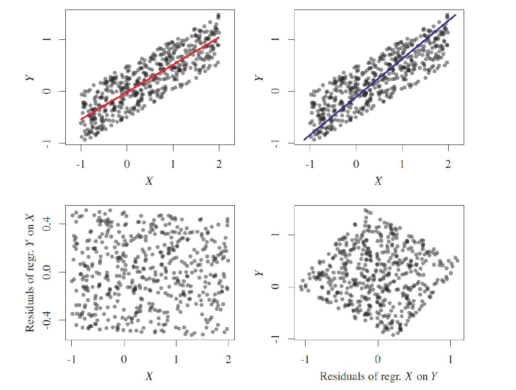Fig 11: Visual representation of residual dependence (right) and independence (left)

Additive Noise Models (ANMs)

We can use other model classes to produce the same identifiability properties of LiNGAMs.

• Nonlinear additive noise models: \(Y := f_y(X) + N_Y \text{, } \perp \!\!\! \perp X\)
• post-nonlinear models: \(Y := g_Y(f_y(X) + N_Y) \text{, } \perp \!\!\!\perp X\)
• discrete non-linear ANMs with either $X$ or $Y \in \mathbb{Z}$

The causal discovery process with ANMs follows the next algorithm:

1. Regress $X$ on $Y$ writing $Y = \hat{f}_Y(X) + N_Y$
2. Test the residuals $N_Y = Y - \hat{f_Y(X)}$ for independence of $X$
3. Repeat steps 1 and 2 with the roles of $X$ and $Y$ interchanged
4. If independence is accepted in one direction and rejected in the other, accept the former as the correct causal one

Information-Geometric Causal Inference (IGCI)

The idea of this method is to leverage the independence between cause and mechanisms by quantifying the shared information between them. If $p(x)$ and $f$ are chosen independently, then $p(y)$ contains information about $f$ and consequently $f^{-1}$. This concept is illustrated in the following graph. Visually, we cannot directly match the distribution of $x$ to any point of $f$; they appear independent. However, it’s evident that the peak in the distribution of $y$ aligns with the portion of small slope in $f$.

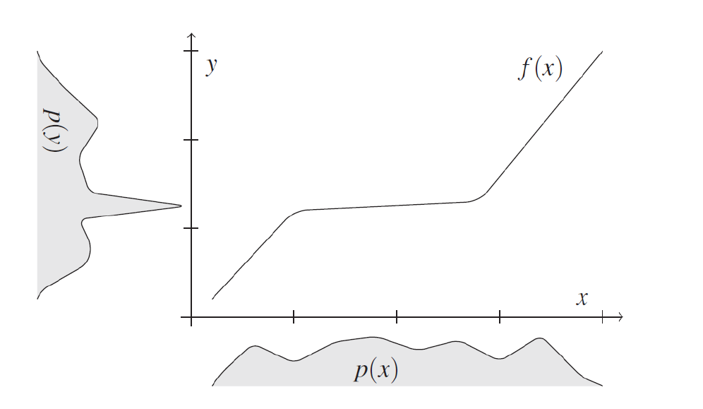Fig 12: Graph Example

IGCI Definition

$P_{X,Y}$ is said to satisfy an IGCI model from $X$ to $Y$ if the following holds:

• $Y=f(X)$ for some diffeomorphism $f$ of $[0, 1]$ that is strictly monotonic and satisfies $f(0)=0$ and $f(1)=1$
• $P_X$ has the strictly positive continuous density $p_X$, such that

\[\begin{equation} \text{cov}[\log f', p_X] = 0 \label{eq:cov} \end{equation}\]

where $\log f’$ and $p_X$ are considered as random variables on the probability space $[0, 1]$ endowed with the uniform distribution

diffeomorphismis when a function is differentiable and bijective and it’s inverse is differentiable.

Theorem: Identifiability of IGCI models

Assume the distribution $P_{X,Y}$ admits and IGCI model from $X$ to $Y$. Then the inverse function $f^{-1}$ satisfies

\[\begin{equation} \text{cov}[\log f^{-1}, p_Y] \ge 0 \label{eq:cov_igci} \end{equation}\]

with equality if and only if $f$ is the identity.

Learning Multivariate Causal Models

Two main approaches for learning causal models from observational data alone:

1. Independence tests → normally just gets to the Markov Equivalence Class
2. Fit restricted model class

Markov Equivalence of Graphs

As indicated in the image, there are three basic graph architectures that compose all other more complex architectures. With independence testing alone, we cannot differentiate between chains and forks because \(X \perp\!\!\!\perp Z | Y\) in both. The only structure that can be identified is the collider, because it is the only one where \(X \not \perp\!\!\!\!\!\perp Z | Y\). Therefore, colliders are the only structures from which we can infer the causal direction with observational data.

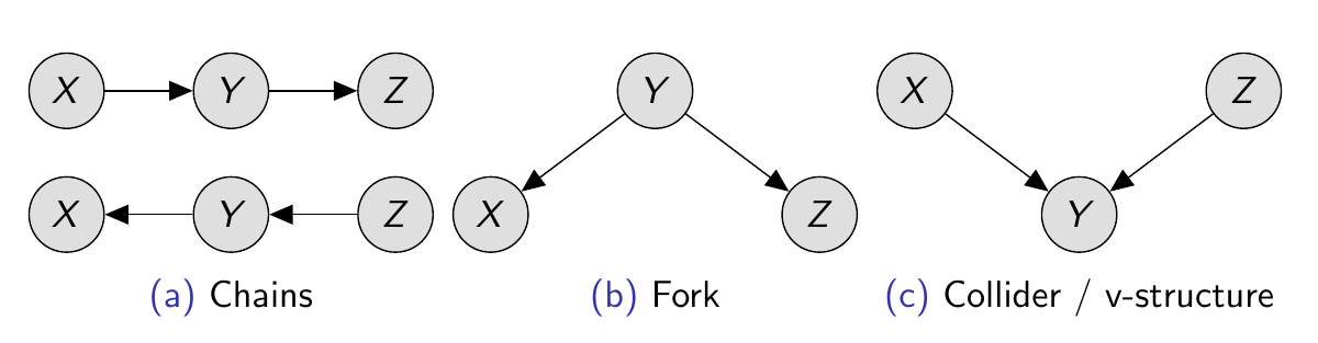Fig 13: The three basic graph architectures in causal graphs

Therefore, we can conclude that observational data alone provides us with a family of causal graphs known as Markov Equivalence Class. The graphs within this class are termed Markov equivalent, and they share the same skeleton (undirected edges) and colliders (with directed edges).

Faithfulness

Faithfulness is a valuable assumption that posits that $p$ is faithful to $G$ if the only (conditional) independencies satisfied by $p$ are those implied by $G$ (via d-separation).

In essence, Faithfulness acts as the counterpart to the Markov condition. While the Markov condition enables us to deduce probabilities from a graph, the faithfulness assumption enables us to infer the graph from probabilities.

It’s worth noting that the Faithfulness assumption may be violated in extreme cases, which typically require deliberate design, so it’s commonly assumed that such cases do not occur naturally.

Score-Based Causal Discovery

Assign a score to each graph $G$ from a set of candidate graphs within the Markov Equivalence Class.

The score $S$ is supposed to reflect how well $G$ explains the observed data $D_{x_1, \dots, x_m }$

\[\begin{equation} \hat{G}=\arg\max_G S(G|D) \label{eq:score_based} \end{equation}\]

The drawback is the exponential search space; e.g., the number of DAGs for $n=5$ and $n=10$ nodes is $29281$ and $4175098976430598143$

Learning from Sparse Domain Shifts

The underlying concept here is that if we possess a dataset in which we are aware that interventions have been conducted (even though we may not know the specifics or locations), this knowledge can aid us in identifying the causal graph.

Given a dataset $\mathcal{D}^e\sim P^e_X$ over observables $X = { X_1, \dots, X_d}, resulting from soft interventions on an unknown subset $\mathcal{I}^e$:

\[\begin{equation} P^e_X(X_1, \dots, X_d) = \color{red}\Pi_{j \in \mathcal{I}^e} P^e_X(X_j|Pa_j) \color{black} \Pi_{j \in [d] \ \mathcal{I}^e} P_X(X_j|Pa_j) \label{eq:domain_shifts} \end{equation}\]

where the first product (red) represents the changed mechanisms. With the Sparse Mechanisms Shift Hypothesis, it can be demonstrated that if we observe all variables $X$ and have sufficiently many environments, we can retrieve the true DAG.

The Sparse Mechanisms Shift Hypothesis posits that distribution shifts occur due to changes in only a subset of the causal model’s mechanisms. For instance, turning off the light affects the entire pixel space, but the distribution shift is primarily caused by changes in the luminance mechanism.

Causal Inference by Using Invariant Predictions

Similar to Dr. Kügelgen, to introduce this idea I’ll leave a quote from Peters et al. (2016)

What is the difference between a prediction that is made with a causal model and that with a non-causal model? Suppose that we intervene on the predictor variables or change the whole environment. The predictions from a causal model will in general work as well under interventions as for observational data. […] We propose to exploit this invariance of a prediction under a causal model for causal inference.

We can frame the problem as a question: “Which of $d$ predictors of $X$ are the causal parents of target variable $Y$?”

Fig 14: Different environments created by multiple interventions

If we assume that we are given data from different environments/interventions:

\[\begin{equation} (X^e,Y^e) \sim P_{X^e, Y^e} \text{for} e\in\mathcal{E} \label{eq:envs} \end{equation}\]

Provided $Y$ was not intervened on, its parents are invariant predictors,

\[\begin{equation} P_{Y^e|PA^e_Y} = P_{Y^f|PA^f_Y} \forall e, f \in \mathcal{E} \label{eq:inv_parents} \end{equation}\]

If we consider the collection $\mathcal{S}$ of all sets $S \subset { 1, \dots, d}$ of variables leading to invariant prediction (at a significance level $\alpha$)

\[\begin{equation} P_{Y^e|PA^e_\mathcal{S}} = P_{Y^f|PA^f_\mathcal{S}} \forall e, f \in \mathcal{E} \text{ and } \forall S \in \mathcal{S} \label{eq:inv_pred} \end{equation}\]

Then the variable appearing in all $S \in \mathcal{S}$ are direct causes of $Y$ with high probability $(1- \alpha)$.

Causal Time Series and Granger Causality

Multivariate time series $(X_t)_{t\in\mathbb{Z}}$ as stationary stochastic process.

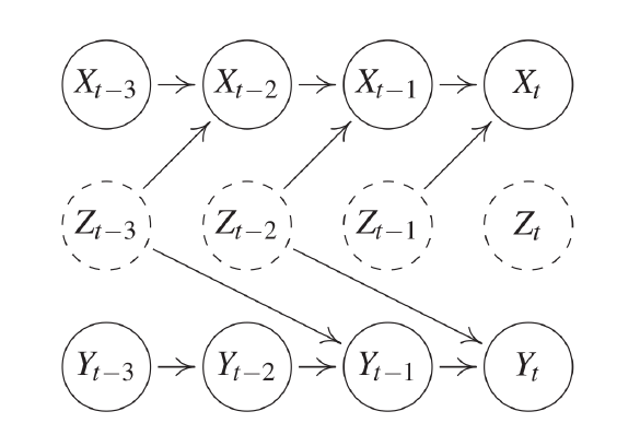Fig 15: Time-based causal graph

By hiding the time variable, we can collapse the same graph in the following form:

Fig 16: Collapsed for of time-based causal graph

Granger Causality

In Granger Causality, we try to figure out which way the cause and effect go by looking at when events happen and if they’re related. We usually think that if something happens first, it’s probably the cause. But sometimes, like when a rooster crows before sunrise, things don’t follow this pattern.

Thought: It’s interesting that when we use really good predictors, they might actually predict what’s going to happen before it does.

Granger Causality ← Conditional (In)dependence + Direction of Time (No intervention needed!)

“X has causal influence on Y whenever past values of X help in predicting Y from its own past”

\[\begin{equation} X \text{ Granger causes } Y \leftrightarrow Y_t \not \perp \!\!\!\!\! \perp X_{past(t)}|X_{past(t)} \label{eq:granger} \end{equation}\]

Practically, this means fitting two regression models, e.g. linear case, and compare the variances of the independent terms (e.g. $N_t$ and $M_t$)

$Y_t = \sum_{i=1}^q a_iY{t-1} + N_t$

$Y_t = \sum_{i=1}^q a_iY{t-1} + \sum_{i=1}^q a_iX{t-1} + M_t$

The issue with this method, and the reason why we emphasize that this is Granger Causality and not regular causality, is that it comes with several limitations due to addressing such a complex problem.

Limitations: Hidden Confounders

Granger causality is more prone to confounding factors, so it’s crucial to adjust for all relevant variables. The multivariate version of Granger Causality is defined as follows:

\[\begin{equation} X^j \text{ Granger-causes } X^k \leftrightarrow X^k_t \not \perp \!\!\! \!\!\perp X^j_{past(t)} | X^{-j}_{past(t)} \label{eq:granger_multi} \end{equation}\]

Because of this, confounders can now affect variables at different time steps, as illustrated in the following image:

Fig 17: Variable Z confounding X and Y in a causal time-series

A real world example where this happens is $X$ being the price of butter, $Y$ the price of cheese and $Z$ the price of milk.

Limitations: Deterministic Relations

Determinism introduces additional independences, which is problematic for conditional independence-based causal inference. In the following example, granger causality infers that there is no causal influence from $X$ to $Y$ nor $Y$ to $X$

Fig 18: Causal time-series graph with deterministic dependences

Limitations: Instantaneous Effects

If the time resolution is not fine enough, “instantaneous” effects of the form $X_t \rightarrow Y_t$ may not be detected by Granger Causality. In the following graph, for example, Granger causality fails to identify the “instantaneous” causal effect.

Fig 18: Causal time-series graph with instantaneous effects

Connections to Machine Learning

In practice, causal inference from finite data needs methods that can do:

• regression, i. e. estimate a function such as a conditional mean: $\mathcal{E}[Y|X=x, do(T=t)] \approx \hat{f}(x,t)$. e.g. for regression adjustment or propensity score weighting
• (conditional) density estimation, $z^{(1)}, \dots, z^{(m)} \sim P^*(Z) \approx P_\theta(Z)$. e.g. for covariate adjustment or assessing overlap

Other applications include kernel-based conditional independence tests for constrained-based causal discovery

Causal Models provide a factorization of complex systems into independent and autonomous modules. This can be helpful for:

• extracting shared information from unlabelled data, e.g. semi-supervised learning
• adapting to distribution shifts, e.g. in domain adaption
• transferring knowledge e.g. in continual or multi-task learning
• planning and reasoning e.g., in algorithmic fairness, recourse, interpretability or explainability

Semi-Supervised Learning (SSL)

In semi-supervised learning (SSL), we utilize a model trained on a small portion of labeled data to label the remaining unlabeled data. Subsequently, with this newly labeled data, we retrain the model. While this practice may seem peculiar, studies have shown that it can sometimes enhance the performance of the model. By employing a causal framework to comprehend the problem, we can argue that SSL only works effectively when the prediction $P_{Y|X}$ is conducted in the anti-causal direction $Y \rightarrow X$, and we can demonstrate that it should not work in the causal direction.

Domain Adaptation & Covariate Shift

In the domain adaptation setting we are given labeled data from a source distribution $(X^S, Y^S) \sim P_{X^S,Y^S} =:P^S$ and wish to make predictions for a target distribution $P^T$ for which only unlabelled data is available $X^T\sim P_{X^T}$.

A common assumption is the covariate shift: $P_{X^S} \neq P_{X T} \text{, but } P_{Y^S|X^S} = P_{Y^T|X^T} =: P_{Y|X}$.

According to the independence of cause and mechanism, this is only justified in a causal learning setting, $X \rightarrow Y$, where a change in $P_X$ does not influence or inform $P_{Y|X}$.

Invariant Models for Causal Transfer Learning

Consider different transfer learning tasks:

• Domain Generalization: Tested in a different domain than trained.
• Multi-task learning: Tested in all domains it was trained
• Asymmetric multi-task learning: Tested in one of the trained domains.

Next, let’s relax the covariate shift assumption to hold only for a subset of variables \(S^*\) which are invariant for prediction. It has been proved that in this set-up, prediction $Y$ using only $X_{S^*}$ is optimal in an adversarial setting.

Algorithmic Fairness

Let A be a protected/sensitive attribute (e.g. race, sex, age, religion)

How can we know that a predictior $\hat{Y} = h(X,A)$ discriminates based on A? $\hat{Y}$ is counterfactually fair if the prediction had not changed has the protected attribute A taken on a different value $a’$ instead of $a$, i.e. if

\[\forall x, a, a': P(\hat{Y}_{A\leftarrow a'}|X=x, A=a) = P(\hat{Y}_{A\leftarrow a}|X=x, A=a)\]

Algorithmic Recourse

This aims to understand the reasons behind a particular event and to determine what actions could have been taken differently to achieve a different outcome. For instance, why was the loan application of individual $x^F$ rejected by the ML model $h$? What steps could have been taken to obtain a more favorable result?

This is formulated as a counterfactual/interventional optimization problem:

\[\min_a \text{cost}(a) \text{ subject to } h(x^F_{d(a)}) > 0.5\]

Denoising by Half-Sibling Regression

If we have a sensor with systematic noise in the measurements, we can denoise it without needing to calibrate it. We can utilize the information from other measurements corrupted by the same systematic noise (referred to as ‘half-siblings’) to denoise the signal of interest.

In this setting, the generation mechanisms of $X$ and $Y$ should be the one represented in the following graph.

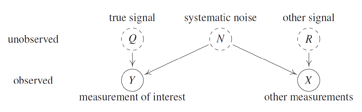Fig 19: Causal graph of noisy sensor

As we can see, all the information shared between $X$ and $Y$ is generated due to the noise $N$, so we can estimate: $\hat{Q}:= Y - \mathcal{E}[Y|X]$

Causal Representation Learning

In this section, Dr. Kügelgen suggests that Causal Representation Learning is akin to Classical Causal Inference as Machine Learning is to Classical AI, for the following reasons:

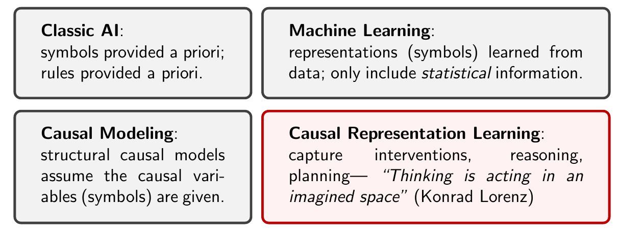Fig 20: Diagram comparing ML and CRL with its “predecessors”

The following image also effectively categorizes the various causal learning tasks:

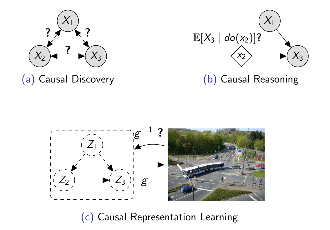Fig 21: Diagram representing Causal Discovery, Causal Reasoning and CRL

CRL: Formalization

Goal: Given $X=f(V)$, recover $(V_1, \dots, V_n)$ and their causal graph G

As a special case, if G is known to empty/trivial, reduces to Independent Component Analysis (ICA)

The challenge with this is that the solution is often highly non-unique, implying that the model is not identifiable. This typically necessitates additional assumptions and/or rich non-i.i.d data to address.

Multi-Domain Data as an Interesting Learning Signal

To address the problem previously outlined, the concept is to gather multiple datasets from various domains or environments. We can conceptualize these different environments as resulting from interventions in a shared causal model. With this perspective, we can identify the true graph by searching for representations $Z$ with sparse mechanism changes.

Fig 22: Diagram representing multi environments represented by interventions

Summary

In the end, Dr. Kügelgen reinforces four important remarks:

• Causal models are a rich model type, capturing not only observational but also interventional (and counterfactual) distributions arising from manipuations of the system.
• Learning causal models from observational data is hard and requires additional assumptions (e.g. no hidden confounding, additive noise)
• Once we have learned a causal model, we can use it for planning and reasoning about interventions and counterfactuals.
• Important limitations and exciting future direction: combine the principle framework of causal modeling with ML strengths in learning representations of complex, high-dimensional data

In my view, the class provided a solid introduction to Causal Inference, covering all the important definitions necessary to understand the theoretical foundations of causality. However, when it came to the practical intersection of Causal Inference and Machine Learning, the discussion felt somewhat superficial. This may be because the field is still in its early stages, leaving much to explore.

After the class, I’ve been considering some potential directions for further exploration, particularly focusing on causal learning based on interventions and causal recourse. These areas seem promising, especially for applications in robotics and reinforcement learning. Unfortunately, these topics weren’t covered extensively in the class, so I’ll need to seek additional material elsewhere.

Dr. Kügelgen also suggested looking into Dr. Barenboim’s work on Causal Reinforcement Learning, which could be a useful next step in my learning journey.